Model Visualization

MiniTorch includes an interactive neural-network explorer built with React Flow. It renders every dense-layer neuron and the complete connection mesh in a standalone HTML file.

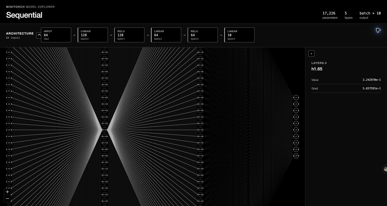
Run the repository example from the project root:

uv run python examples/model_visualization.py

Visualize a model

import numpy as np

from MiniTorch import Variable, sum as tensor_sum
from MiniTorch import visualize
from MiniTorch.nn import Linear, ReLU, Sequential

model = Sequential(
    Linear(784, 256),
    ReLU(),
    Linear(256, 128),
    ReLU(),
    Linear(128, 10),
)

# Capture a concrete activation value and retain its backward gradient.
probe = Variable(np.random.default_rng(7).normal(size=(1, 784)).astype(np.float32))
probe_output = model(probe)
probe_loss = tensor_sum(probe_output)
probe_loss.backward(retain_grad=True)

visualize(model)

This creates model_architecture.html and opens it in the default browser.

Use a custom path or prevent automatic opening:

result = visualize(
    model,
    filename="artifacts/mnist-model.html",
    input_shape=(None, 784),
    open_browser=False,
)

print(result.path)

The neuron map supports:

• every neuron in each Linear layer, without sampling;
• every dense connection, rendered efficiently on a canvas;
• a separate compact architecture section;
• map-style dragging, wheel/pinch zooming, zoom controls, and scrollbars;
• a clean black scientific theme;
• independent collapse buttons for the architecture and neuron inspector;
• a two-field inspector containing only the selected neuron's Value and Grad.

Large networks extend the scrollable canvas. Zoom out for an overview, zoom in to read labels, and drag or scroll to move through all neurons.

Select a circle to inspect it. Value is the mean activation for that neuron over the most recent eager batch. Grad is the corresponding mean activation gradient.

Intermediate activation gradients are released by the default fast backward path. Pass retain_grad=True when preparing a model for inspection:

prediction = model(Variable(x_sample))
loss = tensor_sum(prediction)
loss.backward(retain_grad=True)
visualize(model)

Model-size independence

The exporter reads the supplied module tree and parameter shapes; it does not assume a particular example architecture. For instance:

from MiniTorch import visualize
from MiniTorch.nn import Linear, Sequential

small_model = Sequential(Linear(10, 1))
visualize(small_model, filename="small-model.html")

That page contains exactly 10 input neurons, one output neuron, and 10 connections. Deeper Sequential dense models add one full neuron column for each Linear layer.

Rebuild the viewer

The packaged viewer is already included for Python users. Frontend contributors can rebuild it after changing lib/graph-viewer:

cd lib/graph-viewer
npm ci
npm run typecheck
npm run build

Vite writes the production bundle to MiniTorch/visualization/static. Commit the updated JavaScript and CSS so visualize(model) continues to work without Node.js at runtime.

Computation graph debugging

The lower-level autograd graph viewer remains available:

import numpy as np

from MiniTorch import Variable, visualize_graph

x = Variable(np.array([1.0, 2.0]), name="x")
w = Variable(np.array([0.5, -0.5]), name="w")
y = (x * w).sum()
y.backward(retain_grad=True)

visualize_graph(y, filename="autograd-graph.html")

Use visualize(model) to understand model architecture and visualize_graph(variable) to debug an individual autograd computation.