COMPSCI 713 — AI Fundamentals: Exam Preparation
University of Auckland | Semester 1, 2026 | Instructor: Xinyu Zhang
About This Book
This knowledge base is built to help you learn and prepare for the COMPSCI 713 in-course test (Week 7, 60 minutes, 20 marks).
Every concept is explained using the Feynman method: first in plain language with analogies, then formally with math, then applied to real exam questions. The goal is not just memorisation — it’s understanding.
How to Use This Book
- Start with Part 0 — read the exam analysis to understand what’s tested and with what weight
- Work through modules in priority order — 🔴 modules first (A, B, G, F), then 🟠 (D, H), then 🟡 (C, E)
- For each chapter: read the Feynman Draft first to build intuition, then study the formal definitions, then try the practice problems
- Use the English Expression Guide before the test — practise the sentence templates
- Attempt all 3 mock exams under timed conditions (55 min answering)
- Check your cheat sheet — the frequency map chapter has recommendations for what to write on your handwritten A4 page
Exam Format (Sample Test S1 2026)
| Item | Detail |
|---|---|
| Duration | 60 min (5 min reading + 55 min answering) |
| Total marks | 20 |
| Questions | 6 short-answer questions |
| Notes allowed | Double-sided handwritten A4 page |
| Calculators | Not permitted |
| Style | Quality over quantity — concise, clear answers |
Coverage Map (Weeks 2-5)
| Week | Lecture | Topic | Module |
|---|---|---|---|
| W2 | L1 | Symbolic Logic (Propositional + FOL) | A 🔴 |
| W2 | L2 | Logic Neural Networks (LNN) | B 🔴 |
| W3 | L1 | Knowledge Representation (Expert Systems, Ontologies, KG) | C 🟡 |
| W3 | L2 | Knowledge Graphs for AI (TransE, Embeddings, RAG) | D 🟠 |
| W4 | L1 | MYCIN Expert System (Confidence Factors) | E 🟡 |
| W4 | L2 | Decision Trees & Ensembles (Bagging, Boosting) | F 🔴 |
| W5 | L1 | Soft Computing (Fuzzy Logic, Bayesian, Vagueness vs Uncertainty) | G 🔴 |
| — | — | Multi-Agent Systems (Robot Soccer) | H 🟠 |
Priority Legend
- 🔴 必考 (Must-Know): Appeared in sample test with high mark weight
- 🟠 高频 (High Frequency): Appeared in sample test with moderate weight
- 🟡 中频 (Medium): Full lecture topic, not in sample but likely in actual test
真题逐题分析 — Complete Exam Analysis
Course: COMPSCI 713: AI Fundamentals, University of Auckland Instructor: Xinyu Zhang (mid-semester) / Thomas (final exam, partial) Scope: ALL available exam papers — S1 2025 Sample, S1 2025 Actual, S1 2026 Sample, S1 2024 Final Purpose: Question-by-question breakdown for exam preparation
How to Use This Document(使用指南)
- First pass: Skim the tables at the end of each exam section to see topic/mark distribution
- Second pass: Read the Learning Points for your weakest topics
- Third pass: Use the Common Mistakes as a self-check before the exam
- Final review: Jump to Cross-Exam Patterns at the bottom
💡 核心发现: 每一份试卷都考了 Symbolic Logic, LNN, Knowledge Graphs, 和 Decision Trees/Ensembles。这四个是绝对必考项。
Exam Paper 1: S1 2025 Sample Test
Format: 15 marks, 6 questions, 60 minutes (5 reading + 55 answering) Allowed aids: One double-sided handwritten A4 page
Q1 — Symbolic Logic [3 marks]
Question Summary
(a) Propositional Logic — Modus Tollens [~1.5m]
Scenario: A secure facility grants entry only if a person has a valid ID ($I$) AND fingerprint matches ($F$). Rule: $(I \wedge F) \rightarrow E$. Observed: person was NOT granted entry ($\neg E$).
Task: Deduce what must be true about $I$ and $F$.
(b) First-Order Logic [~1.5m]
Task: Write “Not all birds can fly” in FOL using $\text{Fly}(x)$. Give a realistic example.
Expected Answer
(a):
- By Modus Tollens: $(I \wedge F) \rightarrow E$ and $\neg E$ implies $\neg(I \wedge F)$
- By De Morgan: $\neg I \vee \neg F$
- Conclusion: Either the person lacked a valid ID, or the fingerprint didn’t match (or both)
(b):
- FOL: $\neg \forall x , \text{Fly}(x)$, equivalently $\exists x , \neg \text{Fly}(x)$
- Example: “Penguins are birds but cannot fly”
Analysis
| Item | Detail |
|---|---|
| Topic | Symbolic Logic(符号逻辑) |
| Lecture | W2L1 |
| Type | 推理 + 形式化 (Deduction + Formalisation) |
| Difficulty | ★★☆ |
| Keywords | propositional logic, modus tollens, FOL, universal quantifier, negation |
| Exam intent | Can student apply basic inference rules AND translate English → FOL? |
Learning Points(学习要点)
- Modus Tollens 是本课程考试的第一推理模式: $(P \rightarrow Q), \neg Q \vdash \neg P$。务必熟练到条件反射
- “Not all” = $\neg \forall x$: 注意不是 $\forall x , \neg$(后者意为“所有都不“,语义完全不同)
- De Morgan 定律: $\neg(A \wedge B) = \neg A \vee \neg B$,推导结论时经常用到
⚠️ Common Mistake: Writing $\forall x , \neg \text{Fly}(x)$ which means “NO bird can fly” — much stronger than “not all birds can fly.”
Q2 — Logic Neural Networks (LNN) [2 marks]
Question Summary
Scenario: Smart home LNN rule: HeatingOn $\leftarrow$ Cold $\otimes$ AtHome (differentiable AND).
(a) Interpret in natural language. How does it differ from Boolean? [1m]
(b) Compute with Cold = 0.9, AtHome = 0.4. Discuss whether heating activates. [1m]
Expected Answer
(a):
- Natural language: “If it is cold AND someone is at home, turn on the heating.”
- Difference: Boolean AND requires both inputs strictly TRUE (1). LNN’s $\otimes$ works with continuous truth values in $[0, 1]$, producing intermediate results that capture partial truth and enable gradient-based learning.
(b):
- Product t-norm: $0.9 \times 0.4 = 0.36$
- Lukasiewicz: $\max(0, 0.9 + 0.4 - 1) = 0.3$
- Whether heating activates depends on threshold: if $\alpha = 0.3$, yes; if $\alpha = 0.7$, no.
Analysis
| Item | Detail |
|---|---|
| Topic | Logic Neural Networks(逻辑神经网络) |
| Lecture | W2L2 |
| Type | 概念解释 + 计算 (Explain + Compute) |
| Difficulty | ★★☆ |
| Keywords | LNN, soft conjunction, t-norm, product, Lukasiewicz, threshold |
| Exam intent | Why do we need differentiable logic? Can student compute with t-norms? |
Learning Points
- 必背三个 t-norm:
- Product: $a \times b$
- Lukasiewicz: $\max(0, a + b - 1)$
- Godel/min: $\min(a, b)$
- Boolean vs LNN 的关键差异: Boolean 是离散的 {0,1};LNN 是连续的 [0,1],支持梯度下降
⚠️ Common Mistake: Forgetting to discuss the threshold. Computing 0.36 is not enough — you must state what activation decision follows.
Q3 — Knowledge Graph Embeddings [2 marks]
Question Summary
Explain the role of entity/relation embeddings in KG completion. Introduce a common KG inference task with an example.
Expected Answer
- Embeddings: Map entities and relations to dense vectors in continuous space, enabling mathematical operations for reasoning
- Inference task: Link prediction — given $(h, r, ?)$, predict tail entity
- Example: $(Einstein, bornIn, ?) \rightarrow Germany$
Analysis
| Item | Detail |
|---|---|
| Topic | Knowledge Graphs(知识图谱) |
| Lecture | W3L2 |
| Type | 概念解释 + 举例 (Explain + Example) |
| Difficulty | ★☆☆ |
| Keywords | KG embedding, TransE, link prediction, knowledge completion |
Learning Points
- TransE 核心公式: $h + r \approx t$(头实体向量 + 关系向量 ≈ 尾实体向量)
- 三种推理任务: tail prediction $(h, r, ?)$, head prediction $(?, r, t)$, relation prediction $(h, ?, t)$
⚠️ Common Mistake: Confusing “embedding” with “one-hot encoding.” Embeddings are dense, low-dimensional, learned vectors — not sparse indicator vectors.
Exam tip(答题技巧): 永远给具体例子。“(Einstein, bornIn, ?) → Germany” 远比 “it predicts missing links” 好。
Q4 — Embodied AI / Robot Soccer [2 marks]
Question Summary
Robot soccer league: overhead camera, 225 features per frame, team of 5 robots, no inter-robot communication. Describe strategies/collective behaviours.
Expected Answer
Any of (1 mark each, max 2):
- Collective behaviours: passing strategy, interception prediction, passing point value assessment
- Positioning strategies: formations for attack/defense
- Role-based strategies: dynamic role assignment based on game situation
- Centralized control: overhead camera acts as single controller for all 5 robots
Analysis
| Item | Detail |
|---|---|
| Topic | Embodied AI / Multi-Agent Systems(具身AI/多智能体) |
| Lecture | Multi-Agent lecture |
| Type | 知识回忆 (Recall) |
| Difficulty | ★☆☆ |
| Exam intent | Tests lecture attendance — can you name concrete strategies? |
Learning Points
- 三大策略类别: (1) 集体行为 — passing, (2) 位置策略 — formation, (3) 角色分配 — dynamic assignment
- 关键细节: No communication → centralized control via overhead camera → single decision-maker
⚠️ Common Mistake: Being too vague. “They work together” = 0 marks. Name specific strategies.
Q5 — Random Forest / Bagging [3 marks]
Question Summary
Dataset with 225 features.
(a) How are features selected per tree? How many? [2m]
(b) Why is feature bagging a good idea? [1m]
Expected Answer
(a):
- Random subset of features sampled per tree (not all 225)
- Typical: $\sqrt{p} = \sqrt{225} = 15$ features per tree
- Different trees see different feature subsets
(b):
- Prevents trees from being highly correlated (e.g., same dominant feature always at root)
- Decorrelated trees → ensemble averaging reduces variance more effectively
Analysis
| Item | Detail |
|---|---|
| Topic | Decision Trees & Ensembles(决策树与集成方法) |
| Lecture | W4L2 |
| Type | 解释 + 计算 (Explain + Calculate) |
| Difficulty | ★★☆ |
| Exam intent | Tests “why” not just “what” — understanding the purpose of feature bagging |
Learning Points
- $\sqrt{p}$ rule: For $p$ features, sample $\sqrt{p}$ per tree. For 225 features → 15.
- Bagging vs Boosting:
- Bagging → parallel trees → reduces variance
- Boosting → sequential trees → reduces bias
- 两层随机化: (1) Bootstrap sampling of data rows, (2) Random sampling of features. Both reduce correlation.
⚠️ Common Mistake: Confusing bootstrap sampling (random data points) with feature bagging (random features). Both happen in Random Forest; they serve different purposes.
Q6 — MYCIN / Expert Systems [3 marks]
Question Summary
Medical diagnosis scenario using backward chaining. Patient has a runny nose. Possible diagnoses: common cold, allergies, measles. Demonstrate backward chaining reasoning.
Expected Answer
- Backward chaining: Start from hypothesis, work backward to check conditions
- Hypothesis: Common Cold → needs runny nose ✓, fever ?, cough ?
- Hypothesis: Allergies → needs runny nose ✓, sneezing ?, itchy eyes ?
- Hypothesis: Measles → needs runny nose ✓, rash ?, high fever ?
- Ask additional questions to discriminate between hypotheses
- Contrast with forward chaining: start from facts, derive conclusions
Analysis
| Item | Detail |
|---|---|
| Topic | Expert Systems / MYCIN(专家系统) |
| Lecture | W3L1 (Knowledge Representation) |
| Type | 推理过程演示 (Demonstrate reasoning process) |
| Difficulty | ★★☆ |
| Keywords | backward chaining, hypothesis, rule-based reasoning, MYCIN |
| Exam intent | Can student trace backward chaining step by step? |
Learning Points
- Backward chaining 三步法: (1) Start with hypothesis, (2) Check conditions, (3) Ask for missing info
- Forward vs Backward: Forward = data-driven (fact → conclusion); Backward = goal-driven (hypothesis → verify)
- MYCIN 特色: Uses certainty factors (CF) instead of probabilities; backward chaining for diagnosis
⚠️ Common Mistake: Describing forward chaining when asked for backward chaining. Direction matters!
S1 2025 Sample Test — Summary Table
| Q | Topic | Marks | % | Cognitive Level |
|---|---|---|---|---|
| Q1 | Symbolic Logic | 3 | 20% | Apply + Formalise |
| Q2 | LNN | 2 | 13% | Explain + Compute |
| Q3 | KG Embeddings | 2 | 13% | Explain + Exemplify |
| Q4 | Robot Soccer | 2 | 13% | Recall |
| Q5 | Random Forest | 3 | 20% | Explain + Calculate |
| Q6 | MYCIN / Expert Systems | 3 | 20% | Demonstrate reasoning |
| Total | 15 | 100% |
Exam Paper 2: S1 2025 Actual Test
Format: 15 marks, 6 questions, 60 minutes This is the REAL exam that was sat
Q1 — Symbolic Logic [2 marks]
Question Summary
(a) Given $(P \vee Q) \rightarrow R$ and $\neg R$. Apply Modus Tollens. [1m]
(b) Given $\forall x(\text{Cheat}(x) \rightarrow \text{Disqualified}(x))$ and Alice is not disqualified. Conclude about Alice. [1m]
Expected Answer
(a):
- Modus Tollens: $(P \vee Q) \rightarrow R$ and $\neg R$ implies $\neg(P \vee Q)$
- By De Morgan: $\neg P \wedge \neg Q$
- Both P and Q must be false
(b):
- Universal instantiation: $\text{Cheat}(\text{Alice}) \rightarrow \text{Disqualified}(\text{Alice})$
- Given $\neg \text{Disqualified}(\text{Alice})$, by Modus Tollens: $\neg \text{Cheat}(\text{Alice})$
- Conclusion: Alice did not cheat
Analysis
| Item | Detail |
|---|---|
| Topic | Symbolic Logic(符号逻辑) |
| Lecture | W2L1 |
| Type | 推理 (Pure deduction) |
| Difficulty | ★★☆ |
| Keywords | modus tollens, disjunction, De Morgan, universal instantiation, FOL |
| Exam intent | Modus Tollens again! Plus combining FOL with propositional reasoning |
Learning Points
- 这道题和 Sample 的区别: Sample 用 $(I \wedge F) \rightarrow E$,Actual 用 $(P \vee Q) \rightarrow R$。结论不同!
- $\neg(A \wedge B) = \neg A \vee \neg B$(至少一个为假)
- $\neg(A \vee B) = \neg A \wedge \neg B$(两个都假)
- FOL + Modus Tollens 组合拳: Universal instantiation 先把 $\forall x$ 具体化为 Alice,再用 Modus Tollens
⚠️ Common Mistake: For $\neg(P \vee Q)$, some students write “$P$ or $Q$ is false” — this is WRONG. BOTH must be false. De Morgan on disjunction gives conjunction of negations.
🔑 关键对比: AND 的否定 → 至少一个假 (disjunction); OR 的否定 → 全部假 (conjunction). 这是必须刻在脑子里的。
Q2 — LNN with Truth Bounds [3 marks]
Question Summary
Scenario: Autonomous vehicle collision alert system. Two sensors:
- Pedestrian detector: $P$ with bounds $[L_P, U_P] = [0.8, 0.9]$
- Obstacle detector: $Q$ with bounds $[L_Q, U_Q] = [0.3, 0.6]$
Rule: Alert $\leftarrow P \vee Q$ (disjunction, not conjunction!)
Alert threshold: $\alpha = 0.7$
(a) Determine alert status [2m]
(b) Why are bounds (instead of point estimates) useful in safety-critical applications? [1m]
Expected Answer
(a):
-
Co-norm for OR (using Lukasiewicz):
- Lower bound: $\min(1, L_P + L_Q) = \min(1, 0.8 + 0.3) = 1.0$
- Upper bound: $\min(1, U_P + U_Q) = \min(1, 0.9 + 0.6) = 1.0$
-
OR result bounds: $[1.0, 1.0]$
-
Since lower bound $1.0 \geq \alpha = 0.7$: Alert ACTIVATES
Alternative (product-based co-norm):
- $P \vee Q = P + Q - P \cdot Q$
- Lower: $0.8 + 0.3 - 0.8 \times 0.3 = 0.86$
- Upper: $0.9 + 0.6 - 0.9 \times 0.6 = 0.96$
- Bounds: $[0.86, 0.96]$, both $\geq 0.7$: Alert ACTIVATES
(b):
- Bounds capture epistemic uncertainty — we know the truth value lies somewhere in the interval
- In safety-critical systems, we can make conservative decisions: if even the lower bound exceeds threshold, we act
- Point estimates hide uncertainty; bounds let us reason about worst-case scenarios
Analysis
| Item | Detail |
|---|---|
| Topic | LNN with Truth Bounds(带真值边界的 LNN) |
| Lecture | W2L2 |
| Type | 计算 + 论述 (Compute + Argue) |
| Difficulty | ★★★ |
| Keywords | LNN, truth bounds, co-norm, disjunction, safety-critical, epistemic uncertainty |
| Exam intent | Can student compute with bounds (not just point values)? Understands safety implications? |
Learning Points
- 这是 LNN 的升级版考法: Sample 考 AND 的点值计算,Actual 考 OR 的区间计算
- AND vs OR t-norm/co-norm:
- AND (t-norm): Product → $a \times b$; Lukasiewicz → $\max(0, a + b - 1)$
- OR (co-norm): Product → $a + b - a \times b$; Lukasiewicz → $\min(1, a + b)$
- Safety-critical reasoning: 用 lower bound 做决策 = 最保守策略
⚠️ Common Mistake: Using AND formula when the question says OR! Read the operator carefully: $\otimes$ = AND, $\oplus$ = OR, $\vee$ = OR.
⚠️ 另一个常见错误: 忘记 bounds 是区间运算。不能只算一个值,要算 [lower, upper]。
Q3 — Knowledge Graphs / TransE [2 marks]
Question Summary
(a) Explain the TransE embedding model [1m]
(b) Write the TransE scoring function [1m]
Expected Answer
(a):
- TransE represents entities and relations as vectors in the same space
- Core idea: for a true triple $(h, r, t)$, the head plus relation should approximate the tail: $h + r \approx t$
(b):
- Scoring function: $f(h, r, t) = |h + r - t|$ (L1 or L2 norm)
- Lower score = more likely to be true
- Training: minimize score for true triples, maximize for false (negative sampling)
Analysis
| Item | Detail |
|---|---|
| Topic | Knowledge Graphs / TransE |
| Lecture | W3L2 |
| Type | 概念 + 公式 (Concept + Formula) |
| Difficulty | ★☆☆ |
| Exam intent | TransE is the simplest and most testable KG model — can you state the formula? |
Learning Points
- TransE 必背: $f(h,r,t) = |h + r - t|$,越小越可能是真三元组
- 与 Sample 的区别: Sample 考概念层面(什么是 embedding),Actual 考公式层面(TransE 具体怎么算)
- 局限性: TransE 无法建模 1-to-N 关系(如一个国家有多个城市)
⚠️ Common Mistake: Writing $h + r = t$ (equality) instead of $h + r \approx t$ (approximation). The model learns to minimize the distance, not enforce exact equality.
Q4 — Decision Trees / CART [2 marks]
Question Summary
What does “greedy” mean in the context of CART (Classification and Regression Trees)?
Expected Answer
- Greedy = at each node, CART picks the locally optimal split (maximum information gain or minimum Gini impurity) without considering future splits
- It does not evaluate all possible tree structures to find the global optimum
- This makes it computationally efficient but potentially suboptimal
- Why greedy? Finding the optimal tree is NP-hard
Analysis
| Item | Detail |
|---|---|
| Topic | Decision Trees(决策树) |
| Lecture | W4L1-L2 |
| Type | 概念解释 (Concept explanation) |
| Difficulty | ★☆☆ |
| Keywords | CART, greedy algorithm, local optimum, information gain, Gini impurity |
| Exam intent | Tests understanding of algorithm design philosophy, not just mechanics |
Learning Points
- “Greedy“三要素: (1) 每步选当前最优 (2) 不回溯 (3) 不保证全局最优
- 为什么接受 greedy?: 找最优树是 NP-hard;greedy 在实践中效果够好
- Ensemble 弥补 greedy: Random Forest 通过多棵 greedy tree 的聚合来逼近更好的解
⚠️ Common Mistake: Saying greedy means “fast.” Greedy is about the optimization strategy (local vs global), not speed.
Q5 — Fuzzy Logic [3 marks]
Question Summary
Contrast traditional (Boolean) logic vs fuzzy logic for the rule: IF athlete is STRONG AND athlete is HEAVY THEN athlete is HAMMER_THROWER
Expected Answer
Traditional Logic:
- STRONG = {yes, no}, HEAVY = {yes, no} → HAMMER_THROWER = {yes, no}
- Sharp boundaries: an athlete is either strong or not
- AND = Boolean AND: both must be true for conclusion to hold
Fuzzy Logic:
- STRONG(x) ∈ [0, 1], HEAVY(x) ∈ [0, 1] → HAMMER_THROWER(x) ∈ [0, 1]
- Gradual membership: “somewhat strong” = 0.6, “very heavy” = 0.9
- AND = t-norm (e.g., min): HAMMER_THROWER ≥ min(0.6, 0.9) = 0.6
- Captures vagueness — no sharp cutoff between “strong” and “not strong”
Analysis
| Item | Detail |
|---|---|
| Topic | Fuzzy Logic / Soft Computing |
| Lecture | W5L1 |
| Type | 对比分析 (Compare & Contrast) |
| Difficulty | ★★☆ |
| Exam intent | Core theme: why do we need fuzzy logic? What problem does it solve? |
Learning Points
- 对比答题模板: 分三行写 — (1) Traditional: binary, (2) Fuzzy: continuous, (3) WHY fuzzy is better for this case
- Fuzzy logic 解决 vagueness: “Strong” 没有明确边界 → 需要 membership function
- 给具体数字: 说 “STRONG(athlete) = 0.6” 比抽象描述好得多
⚠️ Common Mistake: Confusing fuzzy logic with probability. Fuzzy = degree of membership (to what extent is this athlete “strong”?). Probability = likelihood of an event (what’s the chance this athlete wins?).
Q6 — GA / Embodied AI [3 marks]
Question Summary
Design a fitness function for a BigDog walking robot using Genetic Algorithm optimization.
Expected Answer
Fitness function components:
- Distance traveled (primary): $f_1 = d / d_{max}$ — further is better
- Stability (constraint): $f_2 = 1 - \text{angular_deviation} / \text{max_deviation}$ — less wobble is better
- Energy efficiency (secondary): $f_3 = 1 - E_{used} / E_{max}$ — less energy is better
- Penalty: $f_{penalty} = -C$ if robot falls
Combined: $F = w_1 f_1 + w_2 f_2 + w_3 f_3 + f_{penalty}$
Key design considerations:
- Must balance multiple objectives
- Weights reflect priority (distance > stability > efficiency typically)
- Penalties for catastrophic failure (falling) should be large
Analysis
| Item | Detail |
|---|---|
| Topic | Genetic Algorithms / Fitness Function Design(遗传算法/适应度函数设计) |
| Lecture | GA/NEAT lectures |
| Type | 设计题 (Design) |
| Difficulty | ★★★ |
| Keywords | fitness function, multi-objective, GA, embodied AI, BigDog |
| Exam intent | Can student translate a real-world goal into a mathematical optimization objective? |
Learning Points
- Fitness function 设计万能框架: (1) 定义主目标, (2) 加约束, (3) 加惩罚项, (4) 用加权求和合并
- 开放题没有唯一答案: 关键是逻辑自洽 + 覆盖关键方面
- 必须提到权衡: 速度 vs 稳定性 vs 能耗
⚠️ Common Mistake: Only considering one objective (e.g., just distance). Real fitness functions must balance multiple competing goals.
S1 2025 Actual Test — Summary Table
| Q | Topic | Marks | % | Cognitive Level |
|---|---|---|---|---|
| Q1 | Symbolic Logic (Modus Tollens + FOL) | 2 | 13% | Apply + Deduce |
| Q2 | LNN (Truth Bounds + OR) | 3 | 20% | Compute + Argue |
| Q3 | KG / TransE | 2 | 13% | Explain + Formula |
| Q4 | Decision Trees (CART greedy) | 2 | 13% | Explain concept |
| Q5 | Fuzzy Logic | 3 | 20% | Compare & Contrast |
| Q6 | GA / Fitness Function Design | 3 | 20% | Design |
| Total | 15 | 100% |
Exam Paper 3: S1 2026 Sample Test
Format: 20 marks, 6 questions, 60 minutes (5 reading + 55 answering) Note: Marks increased from 15 → 20. Same topics, more depth required.
Q1 — Symbolic Logic [5 marks]
Question Summary
(a) Propositional Logic — with Truth Table [3m]
Same scenario as S1 2025 Sample: $(I \wedge F) \rightarrow E$, given $\neg E$. But now explicitly requires a truth table for full marks.
(b) FOL — Birds [2m]
Same “not all birds can fly” question.
Expected Answer
(a):
Step 1: Truth table for $X \rightarrow E$ where $X = I \wedge F$:
| $X$ | $E$ | $X \rightarrow E$ |
|---|---|---|
| 0 | 0 | 1 |
| 0 | 1 | 1 |
| 1 | 0 | 0 |
| 1 | 1 | 1 |
When $E = 0$ and implication is TRUE: $X$ must be 0. [1 mark]
Step 2: Truth table for $I \wedge F$:
| $I$ | $F$ | $I \wedge F$ |
|---|---|---|
| 0 | 0 | 0 |
| 0 | 1 | 0 |
| 1 | 0 | 0 |
| 1 | 1 | 1 |
$I \wedge F = 0$ when at least one is 0. [1 mark]
Step 3: Conclusion — person either lacked valid ID, or fingerprint didn’t match, or both. [1 mark]
(b):
- $\neg \forall x , \text{Fly}(x)$ [1 mark]
- Example: penguins, ostriches, kiwi (kiwi 特别适合 UoA 的语境!) [1 mark]
Analysis
| Item | Detail |
|---|---|
| Topic | Symbolic Logic |
| Lecture | W2L1 |
| Difficulty | ★★☆ |
| Compared to 2025 | Same scenario, more marks → must show truth table explicitly |
Learning Points
- 2026 版本更重视过程: 3 marks for truth table vs 2025’s ~1.5 marks. Show ALL steps.
- 真值表是得分保障: 即使你能直接用 Modus Tollens 推出结论,画真值表拿更稳的分
💡 策略提示: 5 marks = 25% of total. Spend proportional time (~14 minutes). Don’t rush the truth table.
Q2 — LNN [4 marks]
Question Summary
Same HeatingOn scenario as S1 2025 Sample, but 4 marks (was 2).
(a) Interpret rule + compare with Boolean [2m]
(b) Compute with Cold = 0.9, AtHome = 0.4 [2m]
Expected Answer
Same as S1 2025 Sample Q2 but more detail expected for the extra marks:
- (a): Need deeper comparison — mention gradient-based learning, continuous optimization, partial truth
- (b): Show at least two t-norms, discuss threshold selection, explain practical implications
Analysis
| Item | Detail |
|---|---|
| Topic | LNN |
| Compared to 2025 | Same question, doubled marks → expects more thorough answer |
| Difficulty | ★★☆ |
Learning Points
- More marks = more depth expected:
- 2m version: basic computation + brief threshold mention
- 4m version: multiple t-norms + threshold discussion + why LNN matters for AI
- 安全策略: 写出所有你知道的 t-norm 计算结果,对比它们
Q3 — Knowledge Graph Embeddings [2 marks]
Question Summary
Same as S1 2025 Sample Q3: explain entity/relation embeddings + KG inference task + example.
Expected Answer
Identical to S1 2025 Sample Q3. (See above.)
Learning Points
- 三年不变: 这道题完全一样。说明 KG embedding 是必考的固定题型。
Q4 — Robot Soccer [2 marks]
Question Summary
Same as S1 2025 Sample Q4: overhead camera, 225 features, describe strategies.
Expected Answer
Identical to S1 2025 Sample Q4. (See above.)
Learning Points
- 同样三年不变: Robot Soccer 策略也是固定考点。
Q5 — Random Forest [3 marks]
Question Summary
Same as S1 2025 Sample Q5: feature selection + why feature bagging.
Expected Answer
Identical to S1 2025 Sample Q5. (See above.)
Q6 — Vagueness vs Uncertainty [4 marks]
Question Summary
New question type (not in S1 2025 Sample):
Classify 4 scenarios:
- Patient described as “high risk” → Vagueness
- Security system estimates burglary → Uncertainty
- Student rated “almost excellent” → Vagueness
- Spam filter classifies email → Uncertainty
Expected Answer
| Scenario | Classification | Reasoning |
|---|---|---|
| “high risk” patient | Vagueness | Blurry boundary — what counts as “high”? Degree, not yes/no |
| Alarm/burglary estimate | Uncertainty | Unknown ground truth — did burglary actually happen? |
| “almost excellent” student | Vagueness | Gradual concept — no sharp boundary between “good” and “excellent” |
| Spam filter | Uncertainty | Probabilistic inference — inferring unknown class from features |
Analysis
| Item | Detail |
|---|---|
| Topic | Soft Computing — Vagueness vs Uncertainty |
| Lecture | W5L1 |
| Difficulty | ★☆☆ (if you know the distinction) |
| Exam intent | THE central philosophical distinction of soft computing |
Learning Points
- 万能判断法则:
- Vagueness → “To what degree?” → Fuzzy Logic (membership functions)
- Uncertainty → “How likely?” → Bayesian Reasoning (probabilities)
- 快速测试: 概念边界模糊 → vagueness; 世界状态未知 → uncertainty
- 语言线索: “high”, “almost”, “kind of” → vagueness; “estimate”, “predict”, “classify” → uncertainty
⚠️ Common Mistake: Thinking fuzzy logic handles uncertainty. NO — fuzzy handles vagueness; Bayes handles uncertainty. This is THE most important distinction in W5.
S1 2026 Sample Test — Summary Table
| Q | Topic | Marks | % | Cognitive Level |
|---|---|---|---|---|
| Q1 | Symbolic Logic (truth table + FOL) | 5 | 25% | Apply + Formalise |
| Q2 | LNN (soft AND computation) | 4 | 20% | Explain + Compute |
| Q3 | KG Embeddings | 2 | 10% | Explain + Exemplify |
| Q4 | Robot Soccer | 2 | 10% | Recall |
| Q5 | Random Forest / Bagging | 3 | 15% | Explain + Calculate |
| Q6 | Vagueness vs Uncertainty | 4 | 20% | Classify scenarios |
| Total | 20 | 100% |
Exam Paper 4: S1 2024 Final Exam (Thomas’s Section)
Note: This is the final exam (not mid-semester), with questions from a different instructor (Thomas). These topics may or may not appear in 2026’s mid-semester, but they are useful for final exam preparation and general knowledge.
Q1 — Continual Learning [4 marks]
Question Summary
Concept drift, replay methods, Gaussian Mixture Models in continual learning.
Expected Answer
- Concept drift: Data distribution changes over time; model must adapt
- Replay methods: Store subset of old data; replay during training on new data to prevent catastrophic forgetting
- GMM: Can be used to model data distributions; detect drift by comparing distributions
- Stability-plasticity tradeoff: Too much stability → can’t learn new; too much plasticity → forgets old
Analysis
| Item | Detail |
|---|---|
| Topic | Continual Learning(持续学习) |
| Difficulty | ★★☆ |
| Priority for 2026 mid-sem | 🟢 LOW — Thomas’s topic, unlikely in mid-semester |
Q2 — BFS vs UCS [3 marks]
Question Summary
Compare Breadth-First Search and Uniform-Cost Search.
Expected Answer
- BFS: Expands shallowest node first; optimal when all edge costs equal; uses FIFO queue
- UCS: Expands lowest-cost node first; optimal for any non-negative costs; uses priority queue
- Key difference: BFS = optimal for unweighted; UCS = optimal for weighted graphs
Analysis
| Item | Detail |
|---|---|
| Topic | Search Algorithms |
| Priority for 2026 mid-sem | 🟢 LOW — not in Xinyu’s question pattern |
Q3 — MCTS / UCB1 [3 marks]
Question Summary
Explain the components of the UCB1 formula used in Monte Carlo Tree Search.
Expected Answer
$$UCB1 = \bar{X}_j + C \sqrt{\frac{\ln N}{n_j}}$$
- $\bar{X}_j$: average reward of node $j$ (exploitation term)
- $N$: total visits to parent
- $n_j$: visits to node $j$
- $C$: exploration constant
- $\sqrt{\ln N / n_j}$: exploration term — favors less-visited nodes
- Balances exploration vs exploitation
Analysis
| Item | Detail |
|---|---|
| Topic | MCTS / UCB1 |
| Priority for 2026 mid-sem | 🟡 MEDIUM — exploration-exploitation could appear in GA context |
Q4 — RL for Pac-Man [1 mark]
Question Summary
Define state, action, policy, reward for RL applied to Pac-Man.
Expected Answer
- State: Current game board configuration (ghost positions, pellet locations, Pac-Man position)
- Action: Move direction (up, down, left, right)
- Policy: Mapping from state to action (which direction to move in each situation)
- Reward: +10 eating pellet, +200 eating ghost, -500 dying, -1 per time step
Analysis
| Item | Detail |
|---|---|
| Topic | Reinforcement Learning(强化学习) |
| Priority for 2026 mid-sem | 🟢 LOW |
Q5 — GNN [2 marks]
Question Summary
Explain permutation invariance and permutation equivariance in Graph Neural Networks.
Expected Answer
- Permutation invariance: Output doesn’t change when node ordering changes (graph-level prediction)
- Permutation equivariance: Output permutes consistently with input permutation (node-level embeddings)
Analysis
| Item | Detail |
|---|---|
| Topic | Graph Neural Networks |
| Priority for 2026 mid-sem | 🟢 LOW — not in Xinyu’s observed pattern |
Q6 — Self-Supervised Learning [2 marks]
Question Summary
Distinguish pretext tasks from downstream tasks in self-supervised learning.
Expected Answer
- Pretext task: Artificial task designed to learn representations without labels (e.g., predict rotation, fill masked words)
- Downstream task: Actual target task the representations are used for (e.g., classification, NER)
- Relationship: Pretext → learn general features; fine-tune on downstream task with few labels
Analysis
| Item | Detail |
|---|---|
| Topic | Self-Supervised Learning |
| Priority for 2026 mid-sem | 🟢 LOW |
Additional Topics from S1 2024 Final (Answer Key)
The following topics appeared in the S1 2024 final exam answer key:
| Topic | Content | Priority for Mid-Sem |
|---|---|---|
| DQN | Online vs target network, bootstrapping | 🟢 LOW |
| Self-Attention | Q/K/V vectors, advantage over traditional attention | 🟡 MEDIUM |
| LLM System Design | Technical route for LLM-based system | 🟡 MEDIUM |
| Decision Tree vs Forest | Interpretability/efficiency trade-off | 🟠 HIGH (DT is core) |
| Naive Bayes | Conditional independence, feature relevance assumptions | 🟡 MEDIUM |
| NEAT | Mobile robot application, fitness function design | 🟠 HIGH (GA/NEAT is core) |
| Self-Supervised Learning | Pretext/downstream tasks | 🟢 LOW |
| Replay in Continual Learning | Stability-plasticity tradeoff | 🟢 LOW |
| CNN in Self-Driving | CNN application in autonomous vehicles | 🟡 MEDIUM |
Cross-Exam Patterns(跨卷规律总结)
Pattern 1: Repeated Questions(原题重复出现)
以下题目在多份试卷中几乎一模一样地出现:
| Question | S1 2025 Sample | S1 2025 Actual | S1 2026 Sample |
|---|---|---|---|
| $(I \wedge F) \rightarrow E$, $\neg E$ → Modus Tollens | ✅ | variant: $(P \vee Q) \rightarrow R$ | ✅ (with truth table) |
| FOL: “Not all birds can fly” | ✅ | variant: Cheat/Disqualified | ✅ |
| LNN HeatingOn ← Cold ⊗ AtHome | ✅ | variant: Bounds + OR | ✅ |
| KG embeddings + inference task | ✅ | variant: TransE formula | ✅ |
| Robot Soccer strategies | ✅ | — | ✅ |
| Random Forest feature bagging | ✅ | variant: CART greedy | ✅ |
| MYCIN backward chaining | ✅ | — | — |
| Fuzzy logic contrast | — | ✅ | — |
| Vagueness vs Uncertainty | — | — | ✅ |
| GA fitness function | — | ✅ | — |
💡 核心发现: Xinyu 喜欢在 Sample Test 和 Actual Test 之间做微调而非大改。Sample 就是 Actual 的预告片!
Pattern 2: Question Evolution(题目进化路径)
每个核心考点在不同年份有“升级版“:
Symbolic Logic 进化链:
S1 2025 Sample: (I∧F)→E, ¬E → 推理(无真值表要求)
S1 2025 Actual: (P∨Q)→R, ¬R → 推理 + FOL 组合
S1 2026 Sample: 同 2025 Sample 但要求画真值表,5 marks
→ 趋势: 从 “能推理” → “能推理 + 证明过程” → “能推理 + 证明 + 变体”
LNN 进化链:
S1 2025 Sample: 点值计算 (AND), 2 marks
S1 2025 Actual: 区间计算 (OR) + safety reasoning, 3 marks
S1 2026 Sample: 点值计算 (AND), 4 marks (deeper explanation)
→ 趋势: AND 和 OR 交替考,区间 vs 点值交替考
KG 进化链:
S1 2025 Sample: "Explain embeddings" (概念)
S1 2025 Actual: "Write TransE formula" (公式)
S1 2026 Sample: "Explain embeddings" (概念, 同2025 Sample)
→ 趋势: 概念和公式交替考。两手都要准备。
Pattern 3: Mark Allocation Trends
| Topic | 2025 Sample (15m) | 2025 Actual (15m) | 2026 Sample (20m) |
|---|---|---|---|
| Symbolic Logic | 3m (20%) | 2m (13%) | 5m (25%) |
| LNN | 2m (13%) | 3m (20%) | 4m (20%) |
| KG | 2m (13%) | 2m (13%) | 2m (10%) |
| Decision Trees/RF | 3m (20%) | 2m (13%) | 3m (15%) |
| Soft Computing/Fuzzy | — | 3m (20%) | 4m (20%) |
| Embodied AI/GA | 2m (13%) | 3m (20%) | 2m (10%) |
| Expert Systems | 3m (20%) | — | — |
Key insight: Symbolic Logic + LNN consistently take 35-45% of total marks. These two topics alone are worth nearly half the exam.
Pattern 4: Cognitive Level Distribution
| Level | Description | Typical % |
|---|---|---|
| Recall | Name strategies, list features | ~15% |
| Explain | Describe how/why something works | ~30% |
| Compute | Calculate t-norm, truth table, $\sqrt{p}$ | ~25% |
| Compare | Fuzzy vs Boolean, vagueness vs uncertainty | ~15% |
| Design | Fitness function, system strategy | ~15% |
Topic Priority Matrix for 2026 Mid-Semester(2026 期中复习优先级)
Based on cross-exam analysis, here is the definitive priority ranking:
| Priority | Topic | Expected Marks | Study Time |
|---|---|---|---|
| 🔴 MUST | Symbolic Logic (Modus Tollens + truth table + FOL) | 4-5m | 20% |
| 🔴 MUST | LNN (AND/OR, point/bounds, t-norm/co-norm) | 3-4m | 20% |
| 🔴 MUST | Knowledge Graphs (TransE, embeddings, inference) | 2m | 10% |
| 🔴 MUST | Decision Trees & Random Forest (greedy, bagging, $\sqrt{p}$) | 2-3m | 10% |
| 🔴 MUST | Soft Computing (vagueness vs uncertainty, fuzzy vs Boolean) | 3-4m | 15% |
| 🟠 HIGH | Embodied AI / Robot Soccer (strategies, centralized control) | 2m | 8% |
| 🟠 HIGH | GA / NEAT (fitness function design) | 2-3m | 10% |
| 🟠 HIGH | Expert Systems / MYCIN (backward chaining) | 0-3m | 5% |
| 🟡 MEDIUM | Naive Bayes (conditional independence) | 0-2m | 2% |
Exam Strategy Recommendations(应试策略建议)
Time Management(时间分配)
For a 20-mark, 55-minute exam:
- ~2.75 minutes per mark
- Q1 (5m): ~14 minutes
- Q2 (4m): ~11 minutes
- Q3 (2m): ~5.5 minutes
- Q4 (2m): ~5.5 minutes
- Q5 (3m): ~8 minutes
- Q6 (4m): ~11 minutes
Cheatsheet Priorities(A4 速查表优先写什么)
Your double-sided A4 page should include (in order of priority):
- Truth table templates — implication, AND, OR truth tables pre-drawn
- Modus Tollens + De Morgan — write the formulas
- T-norm / Co-norm formulas — all 3 variants for AND and OR
- LNN bounds computation — interval arithmetic rules
- TransE formula — $f(h,r,t) = |h + r - t|$
- $\sqrt{p}$ formula — for Random Forest feature bagging
- Vagueness vs Uncertainty — decision table with examples
- Backward vs Forward chaining — one-line definitions
- Fitness function template — multi-objective weighted sum
- Key FOL patterns — $\neg \forall x = \exists x \neg$
Answer Writing Tips(答题技巧)
- Show your work: 2026 version gives more marks for process (truth tables, step-by-step computation)
- Give concrete examples: “(Einstein, bornIn, ?) → Germany” > “it predicts missing links”
- Use the scenario: Refer back to the specific context (smart home, autonomous vehicle, etc.)
- Label your steps: “Step 1: … Step 2: … Therefore: …”
- Quality over quantity: The exam explicitly states this. Be concise and precise.
- When asked “why”: Give the mechanism, not just the outcome. “Feature bagging decorrelates trees, making ensemble averaging more effective at reducing variance.”
Appendix: Complete Question Index(完整题目索引)
For quick reference, every question across all papers:
| Paper | Q# | Marks | Topic | Key Task |
|---|---|---|---|---|
| 2025 Sample | Q1 | 3 | Symbolic Logic | Modus Tollens + FOL |
| 2025 Sample | Q2 | 2 | LNN | AND computation |
| 2025 Sample | Q3 | 2 | KG | Embeddings + inference |
| 2025 Sample | Q4 | 2 | Robot Soccer | List strategies |
| 2025 Sample | Q5 | 3 | Random Forest | Feature bagging |
| 2025 Sample | Q6 | 3 | MYCIN | Backward chaining |
| 2025 Actual | Q1 | 2 | Symbolic Logic | Modus Tollens (OR variant) + FOL |
| 2025 Actual | Q2 | 3 | LNN | Bounds + OR + safety |
| 2025 Actual | Q3 | 2 | KG / TransE | TransE formula |
| 2025 Actual | Q4 | 2 | Decision Trees | CART greedy |
| 2025 Actual | Q5 | 3 | Fuzzy Logic | Boolean vs Fuzzy |
| 2025 Actual | Q6 | 3 | GA / BigDog | Fitness function design |
| 2026 Sample | Q1 | 5 | Symbolic Logic | Truth table + FOL |
| 2026 Sample | Q2 | 4 | LNN | AND computation (deeper) |
| 2026 Sample | Q3 | 2 | KG | Embeddings + inference |
| 2026 Sample | Q4 | 2 | Robot Soccer | List strategies |
| 2026 Sample | Q5 | 3 | Random Forest | Feature bagging |
| 2026 Sample | Q6 | 4 | Vagueness vs Uncertainty | Classify 4 scenarios |
| 2024 Final | Q1 | 4 | Continual Learning | Concept drift + replay |
| 2024 Final | Q2 | 3 | Search | BFS vs UCS |
| 2024 Final | Q3 | 3 | MCTS | UCB1 formula |
| 2024 Final | Q4 | 1 | RL | State/action/policy/reward |
| 2024 Final | Q5 | 2 | GNN | Permutation invariance |
| 2024 Final | Q6 | 2 | Self-Supervised | Pretext vs downstream |
考点频率分布 — Topic Frequency Heat Map
基于全部可用考试卷的统计分析(S1 2025 Sample, S1 2025 Actual, S1 2026 Sample, S1 2024 Final)
📊 考点频率总览
| 知识模块 | 出现次数 | 总分占比 | 优先级 | 考查形式 |
|---|---|---|---|---|
| Symbolic Logic (PL + FOL + Modus Tollens) | 4/4 卷 | 13-25% | 🔴 必考 | 推理推导 + FOL 翻译 |
| Logic Neural Networks (Soft Logic + Truth Bounds) | 3/3 mid-tests | 13-20% | 🔴 必考 | 计算 + 概念对比 |
| Knowledge Graphs (TransE + Embeddings + Inference) | 3/3 mid-tests | 10-13% | 🔴 必考 | 概念解释 + 公式 |
| Decision Trees & Ensembles (CART + RF + Bagging) | 3/4 卷 | 10-20% | 🔴 必考 | 概念理解 + 应用 |
| Soft Computing (Fuzzy Logic + Vagueness vs Uncertainty) | 3/4 卷 | 15-20% | 🔴 必考 | 对比分析 + 场景分类 |
| NEAT & Genetic Algorithms | 2/4 卷 | 13-20% | 🟠 高频 | 适应度函数设计 |
| Embodied AI & Robot Soccer | 2/3 mid-tests | 10-13% | 🟠 高频 | 策略描述 |
| MYCIN / Expert Systems (Backward Chaining) | 1/3 mid-tests | 13-20% | 🟠 高频 | 推理过程描述 |
| Naïve Bayes | 1/4 卷 (final) | ~10% | 🟡 中频 | 假设解释 |
| Knowledge Representation (Frames, Semantic Nets, RBS) | 0 (直接考题) | — | 🟢 低频 | 间接考查 |
🎯 按考题编号统计(Mid-term Test 模式)
每份试卷固定 6 道简答题,主题分布如下:
| 题号 | S1 2025 Sample (15m) | S1 2025 Actual (15m) | S1 2026 Sample (20m) |
|---|---|---|---|
| Q1 | Symbolic Logic (3m) | Symbolic Logic (2m) | Symbolic Logic (5m) |
| Q2 | LNN (2m) | LNN (3m) | LNN (4m) |
| Q3 | Knowledge Graphs (2m) | Knowledge Graphs (2m) | Knowledge Graphs (2m) |
| Q4 | Robot Soccer (2m) | Decision Trees (2m) | Robot Soccer (2m) |
| Q5 | Random Forest (3m) | Fuzzy Logic (3m) | Random Forest (3m) |
| Q6 | MYCIN/Backward Chaining (3m) | GA/Fitness Function (3m) | Vagueness vs Uncertainty (4m) |
规律总结:
- Q1 永远是 Symbolic Logic(分值从 2→5 递增!)
- Q2 永远是 LNN(分值从 2→4 递增!)
- Q3 永远是 Knowledge Graphs / TransE
- Q4-Q6 在以下主题中轮换:Decision Trees/RF、Soft Computing/Fuzzy、NEAT/GA、Robot Soccer、MYCIN
📈 分值趋势分析
2025 Sample (15m):  Logic(3) + LNN(2) + KG(2) + Robot(2) + RF(3) + MYCIN(3)
2025 Actual (15m):  Logic(2) + LNN(3) + KG(2) + DT(2) + Fuzzy(3) + GA(3)
2026 Sample (20m):  Logic(5) + LNN(4) + KG(2) + Robot(2) + RF(3) + V/U(4)
关键发现:
- 2026 总分从 15→20,额外的 5 分主要加在了 Logic (+2) 和 LNN (+2) 上
- Symbolic Logic 要求从“代数推导“升级为“完整真值表“
- Vagueness vs Uncertainty 是新增的高分考点(4分)
⏰ 建议复习时间分配(基于频率和分值)
| 模块 | 建议时间占比 | 理由 |
|---|---|---|
| Symbolic Logic | 20% | 每卷必考,分值最高(最多 5m),需要熟练掌握真值表 + Modus Tollens |
| LNN | 15% | 每卷必考,分值递增,计算和概念并重 |
| Soft Computing (Fuzzy + Bayes + V/U) | 15% | 高频,vagueness vs uncertainty 新增为高分考点 |
| Decision Trees & Ensembles | 15% | 高频,重点理解“为什么“ (greedy, feature bagging) |
| Knowledge Graphs & TransE | 10% | 每卷必考但分值稳定在 2m,概念性强 |
| NEAT & GA | 10% | 高频,重点是 fitness function 设计 |
| Embodied AI & Robot Soccer | 10% | 中频,概念性强,答题灵活 |
| MYCIN & Expert Systems | 5% | 低频但重要概念(backward chaining) |
🧩 考点共现分析
以下概念经常在同一道题或同一考卷中一起出现:
| 概念组合 | 出现模式 | 意义 |
|---|---|---|
| Modus Tollens + De Morgan’s | 每道 Q1 | 先否定后件,再展开否定前件 |
| LNN + Soft Logic AND | 每道 Q2 | LNN 的核心计算依赖 Product-Sum AND |
| LNN Bounds + Safety-Critical | 2025 Actual | bounds 在自动驾驶中的应用 |
| TransE + Link Prediction | 每道 Q3 | h+r≈t 用于预测缺失链接 |
| Fuzzy vs Traditional Logic | 2025 Actual | 同一规则在两种体系下的对比 |
| GA + Embodied AI | 2025 Actual | 用 GA 训练 BigDog 机器人控制器 |
| Vagueness vs Uncertainty | 2026 Sample | 四个场景分类 |
| Bagging + Feature Bagging | 每道 RF 题 | 两者缺一不可 |
🎯 Cheatsheet 优先级排序
根据出题频率和分值,你的双面 A4 手写笔记应该包含以下内容(按重要性排序):
必须写(占据 60% 空间)
- Modus Tollens 公式 + De Morgan’s Laws + 两种 premise 结构的展开方式
- 完整的 implication 真值表 (4 行)
- LNN Soft Logic (Product-Sum): AND = A×B, OR = A+B-AB, NOT = 1-A
- LNN Truth Bounds 分类规则 (L≥α → TRUE, U≤α → FALSE, etc.)
- OR bounds: L=max(L₁,L₂), U=max(U₁,U₂)
- TransE: h+r≈t, f(h,r,t) = ||h+r-t||
- Entropy: H(X) = -Σp(x)log₂p(x), IG = H(Y) - H(Y|X)
- Gini: G(D) = 1 - Σpᵢ²
- Fuzzy: AND=min, OR=max, NOT=1-μ
- Vagueness vs Uncertainty 判断流程图
建议写(占据 30% 空间)
- Bayes’ Theorem: P(H|e) = P(e|H)P(H)/P(e)
- Naïve Bayes: P(C|x) ∝ P(C)ΠP(xᵢ|C)
- CART = greedy (no look-ahead)
- RF = Bagging + Feature Bagging (√features)
- CF(conclusion) = CF(premise) × CF(rule)
- Forward vs Backward Chaining 对比
- NEAT: speciation distance δ = c₁E/N + c₂D/N + c₃W̄
- Flocking 3 rules: separation, cohesion, alignment
如果有空间(占据 10%)
- FOL 量词否定: ¬∀x P(x) ≡ ∃x ¬P(x)
- STEAM: Joint Persistent Goal (A/U/I)
- Ontology vs KG 区别
- RDF triple 格式
命题风格分析 — Teacher Style Analysis
Instructor: Xinyu Zhang | Course: COMPSCI 713 AI Fundamentals | S1 2026 基于全部可用考试卷分析(S1 2025 Sample, S1 2025 Actual, S1 2026 Sample, S1 2024 Final)
👤 教师信息
- Instructor: Xinyu Zhang (School of Computer Science, University of Auckland)
- Course: COMPSCI 713: AI Fundamentals, S1 2026
- Website: zhangxinyu-xyz.github.io
- 另一位出题者: Thomas (负责 Part 2 — 深度学习/RL/LLM 相关,与 Xinyu 的 Part 1 分开考)
🎯 出题风格总结
1. 偏好应用场景题(Application-Based Scenarios)
Xinyu 的题目几乎从不直接问定义。每道题都嵌入在一个具体场景中:
| 场景类型 | 出现频率 | 具体例子 |
|---|---|---|
| 安全/门禁系统 | 3 次 | Secure facility (I∧F→E), smart office alarm (P∨Q→R) |
| 智能家居 | 2 次 | Smart home heating (LNN HeatingOn) |
| 自动驾驶 | 1 次 | Autonomous vehicle collision alert (LNN bounds) |
| 医疗诊断 | 1 次 | Runny nose backward chaining |
| 体育/健身 | 1 次 | Hammer thrower (fuzzy logic) |
| 机器人 | 2 次 | Robot soccer, BigDog walking |
| 金融/商业 | 1 次 | Stock prediction (random forest) |
应对策略:不要死记硬背定义,要练习在新场景中应用概念。
2. 偏好“为什么“而非“是什么“
典型问法:
- “Why is feature bagging considered a good idea?” (不是 “What is feature bagging?”)
- “What exactly is meant by saying CART is ‘greedy’?” (不是 “Define CART”)
- “Why is using bounds beneficial in safety-critical applications?” (不是 “What are bounds?”)
应对策略:准备好每个概念的原因和动机,不仅仅是定义。
3. 重视对比分析(Contrast & Compare)
高频出题模式:
- Boolean logic vs LNN soft logic(每卷 Q2)
- Traditional logic vs Fuzzy logic(2025 Actual Q5)
- Vagueness vs Uncertainty(2026 Sample Q6)
- Decision tree vs Decision forest(2024 Final)
- Forward chaining vs Backward chaining(隐含在 MYCIN 题中)
应对策略:准备好两栏对比表格,考试时直接画表回答。
4. 计算题轻量但必须准确
- LNN: 0.9 × 0.4 = 0.36 这种简单乘法
- Entropy/Gini: 不会给太复杂的数据,但公式必须正确
- TransE: 概念性理解 h+r≈t 即可,不需要实际向量计算
应对策略:把公式写在 cheatsheet 上,考试时代入数字即可。
5. 评分标准:Quality over Quantity
考试说明明确写道:
“We privilege quality over quantity, i.e., you do not need to write very long answers. Be concise and clear.”
| 答题长度建议 | 分值 | 建议写法 |
|---|---|---|
| 1 mark | 1-2 句话 | 一个关键点,直接命中 |
| 2 marks | 3-4 句话或一个小段落 | 两个关键点 + 简短解释 |
| 3 marks | 一个段落或结构化回答 | 三个关键点 + 各自解释 |
| 4-5 marks | 结构化回答 + 例子/表格 | 多个关键点 + 具体例子 + 对比 |
6. 常用句式模式
Xinyu 的题目经常使用以下句式:
- “Use propositional logic to deduce what must be true about X and Y.” → 用 Modus Tollens + De Morgan’s
- “What does this rule represent in natural language, and how is it different from…” → 翻译 + 对比
- “Explain how the LNN would likely compute…” → 写出计算步骤
- “Contrast how the above rule might work using traditional logic as compared to…” → 画对比表
- “For each of the following situations, state whether it is mainly…” → 分类 + 简短理由
- “Describe one strategy or collective behaviour…” → 从课堂内容中选一个,解释清楚
- “Name the elements that should be part of the fitness function…” → 列出 3-5 个关键要素
🔄 题目进化趋势(2025 → 2026)
| 变化维度 | 2025 | 2026 预测 |
|---|---|---|
| 总分 | 15 marks | 20 marks |
| Logic 分值 | 2-3 marks | 5 marks(要求真值表) |
| LNN 分值 | 2-3 marks | 4 marks(更深入) |
| 新增考点 | — | Vagueness vs Uncertainty (4m) |
| 难度 | 中等 | 稍有提升(需要更完整的推导过程) |
| 时间压力 | 55min/15m ≈ 3.7min/mark | 55min/20m = 2.75min/mark |
关键发现:2026 时间更紧了!每分只有 2.75 分钟,比 2025 的 3.7 分钟少了约 25%。必须更加简洁高效。
⚠️ 常见陷阱与扣分点
| 陷阱 | 说明 | 正确做法 |
|---|---|---|
| 混淆 ¬(A∧B) 和 ¬(A∨B) | De Morgan’s 展开方向不同 | ¬(A∧B)=¬A∨¬B, ¬(A∨B)=¬A∧¬B |
| 混淆 vagueness 和 uncertainty | “high risk” 是 vagueness,“is there a burglary?” 是 uncertainty | 问“概念本身有没有模糊边界“ |
| 忘记说 CART 是 “no look-ahead” | 只说 “maximizes impurity reduction” 只能拿一半分 | 必须强调 greedy = no look-ahead |
| LNN 中混淆 Product-Sum 和 min/max | 考题用 Product-Sum AND (A×B),fuzzy 用 min | 看题目指定的是哪种运算 |
| Feature bagging 只说 “random features” | 需要说明目的是 decorrelate trees | 解释为什么:防止 dominant feature 总是做 root |
| Backward chaining 不说 “start from goal” | 关键是从假设出发 | 明确说 “start with hypothesis, find support” |
| TransE 忘记说 “smaller score = more likely” | 这是 distance-based score | f(h,r,t) = ||h+r-t||, 越小越好 |
📝 高分答题策略
1. 结构化回答
对于 2-3 分的题,使用:
[1句总结] + [关键点1 + 解释] + [关键点2 + 解释]
2. 对比题用表格
| Aspect | Method A | Method B |
|--------|---------|---------|
| ...    | ...     | ...     |
3. 计算题写出每一步
Given: Cold = 0.9, AtHome = 0.4
AND (Product-Sum) = 0.9 × 0.4 = 0.36
If threshold α = 0.5, then 0.36 < 0.5 → heating NOT activated
4. 推理题用链式推导
Given: ¬E
Rule: (I ∧ F) → E
By Modus Tollens: ¬E → ¬(I ∧ F)
By De Morgan's: ¬(I ∧ F) = ¬I ∨ ¬F
∴ Either ¬I or ¬F (or both)
5. 时间管理(2026 格式,20 marks / 55 min)
| 题号 | 预期分值 | 建议时间 | 策略 |
|---|---|---|---|
| Q1 (Logic) | 5m | 12 min | 先写代数推导,再补真值表 |
| Q2 (LNN) | 4m | 10 min | 先翻译,再计算,最后对比 |
| Q3 (KG) | 2m | 5 min | TransE 公式 + 一个例子 |
| Q4 (轮换) | 2m | 5 min | 从课堂内容选一个策略展开 |
| Q5 (轮换) | 3m | 8 min | 结构化回答,每个分点一段 |
| Q6 (轮换) | 4m | 10 min | 每个子题 2-3 句,确保覆盖评分点 |
| 检查 | — | 5 min | 检查计算和 De Morgan’s 方向 |
Symbolic Logic – Propositional & First-Order Logic
🎯 Exam Importance
🔴 GUARANTEED TO APPEAR | Every single test paper has a logic question as Q1
| Test Paper | Question | Marks | Sub-topics |
|---|---|---|---|
| S1 2025 Sample Test | Q1 (3 marks / 15 total = 20%) | 1(a) Modus Tollens + De Morgan’s on $(I \wedge F) \rightarrow E$; 1(b) FOL translation $\neg\forall x, \text{Fly}(x)$ + example | |
| S1 2025 Actual Test | Q1 (2 marks / 15 total = 13%) | 1(a) Modus Tollens + De Morgan’s on $(P \vee Q) \rightarrow R$; 1(b) FOL Modus Tollens with $\forall x(\text{Cheat}(x) \rightarrow \text{Disqualified}(x))$ | |
| S1 2026 Sample Test | Q1 (5 marks / 20 total = 25%) | 1(a) Same $(I \wedge F) \rightarrow E$ but requires full truth table (3 marks); 1(b) Same FOL $\neg\forall x, \text{Fly}(x)$ |
Key observation: The question has been worth 2–5 marks across papers, and the 2026 sample tripled the propositional logic marks by requiring a full truth table. Prepare for both approaches (algebraic deduction AND truth table verification).
📖 Core Concepts (Quick Reference Table)
| English Term | 中文 | One-line Definition |
|---|---|---|
| Propositional Logic(命题逻辑) | 命题逻辑 | Deals with statements that are TRUE or FALSE, combined with logical connectives |
| First-Order Logic / FOL(一阶逻辑) | 一阶逻辑 | Extends propositional logic with variables, quantifiers ($\forall$, $\exists$), predicates, and functions |
| Atomic Proposition(原子命题) | 原子命题 | A basic statement with binary value: true or false (e.g., “It is raining”) |
| Connective(逻辑联结词) | 联结词 | Operators: $\neg$ (NOT), $\wedge$ (AND), $\vee$ (OR), $\rightarrow$ (IMPLIES), $\leftrightarrow$ (IFF) |
| Interpretation(解释/赋值) | 解释 | A function $\pi$ that assigns true/false to every atomic proposition |
| Tautology(重言式) | 重言式 | A formula that is true under every possible interpretation |
| Logical Implication(逻辑蕴含) | 逻辑蕴含 | $A \Rightarrow B$: for every interpretation where A is true, B must also be true |
| Logical Equivalence(逻辑等值) | 逻辑等值 | $A \Leftrightarrow B$: A and B have the same truth value under every interpretation |
| Modus Ponens(肯定前件) | 肯定前件 | From $P$ and $P \rightarrow Q$, conclude $Q$ |
| Modus Tollens(否定后件) | 否定后件 | From $P \rightarrow Q$ and $\neg Q$, conclude $\neg P$ |
| Syllogism(三段论) | 三段论 | From $(A \rightarrow B)$ and $(B \rightarrow C)$, conclude $(A \rightarrow C)$ |
| Material Implication(实质蕴含) | 实质蕴含 | $A \rightarrow B$ is false ONLY when A is true and B is false |
| Vacuous Truth(空真) | 空真 | When the premise is false, implication is always true |
| De Morgan’s Laws(德摩根定律) | 德摩根律 | $\neg(A \wedge B) \equiv \neg A \vee \neg B$ and $\neg(A \vee B) \equiv \neg A \wedge \neg B$ |
| Universal Quantifier(全称量词) | 全称量词 | $\forall x$: “for all x in the domain” |
| Existential Quantifier(存在量词) | 存在量词 | $\exists x$: “there exists at least one x” |
| Bound Variable(约束变量) | 约束变量 | A variable within the scope of a quantifier ($\forall x$ or $\exists x$) |
| Free Variable(自由变量) | 自由变量 | A variable NOT within any quantifier’s scope |
| Sentence(语句) | 语句 | A formula with NO free variables |
| Signature(签名) | 签名 | The vocabulary of a FOL language: its relation and function symbols |
| Domain(论域) | 论域 | The set of objects that variables range over in a FOL interpretation |
🧠 Feynman Draft – Learning From Scratch
Part 1: Propositional Logic
Imagine you are a security guard at a building entrance. Your job manual has simple rules written as “if… then…” statements. Each fact is either TRUE or FALSE – no grey areas, no “maybe.” Your entire job is to follow the rules and figure out what must be true.
For example, your manual says:
“If the person has a valid ID and their fingerprint matches, then grant entry.”
In symbols: $(I \wedge F) \rightarrow E$
Now, suppose today the person was denied entry ($\neg E$). What can you figure out?
Think of it this way: the rule promises that having both ID and fingerprint match guarantees entry. The person was NOT granted entry. So the guarantee must not have kicked in – meaning they did NOT have both. Either no valid ID, or no fingerprint match, or both were missing.
This reasoning is called Modus Tollens(否定后件): if the consequence didn’t happen, the premise couldn’t have been fully satisfied.
$$P \rightarrow Q, \quad \neg Q \quad \Longrightarrow \quad \neg P$$
But wait – what does “not both” mean precisely?
$\neg(I \wedge F)$ means “it’s not the case that BOTH are true.” By De Morgan’s Law, this equals $\neg I \vee \neg F$ – “at least one of them is false.”
This is exactly how every exam question on this topic works. Every. Single. One.
Part 2: The Implication Trap
Here is the single most confusing thing in propositional logic, and the lecture opens with it:
“If it rains today, I will bring an umbrella.” ($P \rightarrow Q$)
You see the person carrying an umbrella ($Q$ is true). Can you conclude it is raining ($P$)?
NO! $Q \rightarrow P$ is NOT the same as $P \rightarrow Q$. The person might just like carrying umbrellas. This mistake is called Affirming the Consequent(肯定后件谬误) – the lecture slide 4-5 opens with exactly this example.
Here is the full truth table for implication:
| $P$ | $Q$ | $P \rightarrow Q$ |
|---|---|---|
| T | T | T |
| T | F | F $\leftarrow$ the ONLY row where it’s false |
| F | T | T $\leftarrow$ vacuous truth |
| F | F | T $\leftarrow$ vacuous truth |
The key insight: $P \rightarrow Q$ is false ONLY when P is true and Q is false.
Why is $\text{false} \rightarrow \text{anything}$ true? Think of it as a promise: “If it rains, I’ll bring an umbrella.” If it doesn’t rain, I haven’t broken my promise regardless of whether I carry an umbrella. The promise is only broken when rain happens and no umbrella appears.
⚠️ Common Misconception: Students think $P \rightarrow Q$ means “P causes Q” or “P and Q are related.” It does NOT. Material implication is purely about truth values. “If pigs fly, then I am the Queen of England” is technically TRUE because the premise is false. This is called vacuous truth(空真).
Part 3: First-Order Logic
Propositional logic treats facts as indivisible boxes – “it is raining” is one atomic unit. But what if you need to say something about many things at once?
Imagine you are a biologist studying birds. You want to express: “Not all birds in this region can fly.” In propositional logic, you would need a separate proposition for each bird – $\text{Fly}(\text{robin})$, $\text{Fly}(\text{kiwi})$, $\text{Fly}(\text{penguin})$, etc. If you have 1000 birds, you need 1000 propositions. This is the verbosity problem(冗余问题).
First-order logic fixes this by introducing:
- Objects: things in your world (birds, people, squares in Wumpus World)
- Predicates (relations): properties of objects ($\text{Fly}(x)$, $\text{Pit}(x,y)$)
- Functions: mappings from objects to objects ($\text{left}(x,y)$, $\text{fatherOf}(x)$)
- Quantifiers: $\forall$ (“for all”) and $\exists$ (“there exists”)
So “Not all birds can fly” becomes simply: $\neg \forall x, \text{Fly}(x)$
Which is equivalent to: $\exists x, \neg\text{Fly}(x)$ – “there exists a bird that cannot fly.”
⚠️ Common Misconception: Students write $\forall x, \neg\text{Fly}(x)$ for “not all birds fly.” This is WRONG – it means “NO bird can fly” (way too strong). The negation must go OUTSIDE the quantifier: $\neg\forall x, \text{Fly}(x)$.
⚠️ Common Misconception: With $\forall$, use $\rightarrow$ (implication) not $\wedge$. “Every student cheats” is $\forall x (\text{Student}(x) \rightarrow \text{Cheat}(x))$, NOT $\forall x (\text{Student}(x) \wedge \text{Cheat}(x))$. The latter says “everything is both a student AND a cheater” – it claims your dog is a cheating student!
💡 Core Intuition: Propositional logic is about combining true/false statements with connectives; FOL adds the power to talk about “all” and “some” objects in a domain using quantifiers and predicates.
📐 Formal Definitions
Propositional Logic – Complete Syntax and Semantics
Syntax (from lecture slide 15):
- Atomic propositions (atoms): $\text{Atom} = {X_1, \ldots, X_k}$, each with domain ${\text{true}, \text{false}}$ (or ${0, 1}$).
- Compound propositions are built using connectives: $\neg A$, $(A \vee B)$, $(A \wedge B)$, $(A \rightarrow B)$, $(A \leftarrow B)$, $(A \leftrightarrow B)$
Semantics:
An interpretation $\pi : \text{Atom} \rightarrow {\text{true}, \text{false}}$ assigns truth values to all atoms. The truth value of any compound proposition is determined by the following table:
Master Truth Table (MEMORIZE THIS)
| $A$ | $B$ | $\neg A$ | $A \wedge B$ | $A \vee B$ | $A \rightarrow B$ | $A \leftarrow B$ | $A \leftrightarrow B$ |
|---|---|---|---|---|---|---|---|
| T | T | F | T | T | T | T | T |
| T | F | F | F | T | F | T | F |
| F | T | T | F | T | T | F | F |
| F | F | T | F | F | T | T | T |
Key observations:
- $A \rightarrow B$ is false ONLY in row 2 (A true, B false)
- $A \leftrightarrow B$ is true when A and B have the SAME value
- $A \leftarrow B$ is the “reverse implication” ($B \rightarrow A$)
Complete Logical Equivalence Laws (from lecture slide 22)
These are your tools for algebraic manipulation. The exam requires you to cite which law you use.
| Law Name | Equivalence |
|---|---|
| Double Negation | $\neg\neg A \Leftrightarrow A$ |
| Commutative | $(A \wedge B) \Leftrightarrow (B \wedge A)$; $(A \vee B) \Leftrightarrow (B \vee A)$ |
| Associative | $(A \wedge (B \wedge C)) \Leftrightarrow ((A \wedge B) \wedge C)$; same for $\vee$ |
| Distributive | $(A \wedge (B \vee C)) \Leftrightarrow ((A \wedge B) \vee (A \wedge C))$; $(A \vee (B \wedge C)) \Leftrightarrow ((A \vee B) \wedge (A \vee C))$ |
| Idempotent | $(A \wedge A) \Leftrightarrow A$; $(A \vee A) \Leftrightarrow A$ |
| De Morgan’s | $\neg(A \wedge B) \Leftrightarrow (\neg A \vee \neg B)$; $\neg(A \vee B) \Leftrightarrow (\neg A \wedge \neg B)$ |
| Implication | $(A \rightarrow B) \Leftrightarrow (\neg A \vee B)$; $(A \rightarrow B) \Leftrightarrow (\neg A \wedge \neg B) \vee B$ … simplified: $\neg A \vee B$ |
| Contrapositive | $(A \rightarrow B) \Leftrightarrow (\neg B \rightarrow \neg A)$ |
| Contradiction | $(A \vee (B \wedge \neg B)) \Leftrightarrow A$ |
| Absorption | $A \Leftrightarrow (A \wedge (A \vee B))$; $A \Leftrightarrow (A \vee (A \wedge B))$ |
| Equivalence | $(A \leftrightarrow B) \Leftrightarrow ((A \rightarrow B) \wedge (B \rightarrow A))$; $(A \leftrightarrow B) \Leftrightarrow ((A \wedge B) \vee (\neg A \wedge \neg B))$ |
Logical Implication vs. Material Implication
This distinction is subtle and important (lecture slide 21):
- Material implication ($A \rightarrow B$): a connective inside a formula. It has a truth value.
- Logical implication ($A \Rightarrow B$): a meta-statement about formulas. It means: for EVERY interpretation $\pi$, if $\pi(A) = \text{true}$ then $\pi(B) = \text{true}$.
Verification methods:
- Truth table: check that every row where A is true also has B true
- Equivalent test: $A \Rightarrow B$ if and only if $A \rightarrow B$ is a tautology
Key Inference Rules (from lecture slide 21)
$$\text{Modus Ponens: } ((A \rightarrow B) \wedge A) \Rightarrow B$$
$$\text{Modus Tollens: } ((A \rightarrow B) \wedge \neg B) \Rightarrow \neg A$$
$$\text{Syllogism: } ((A \rightarrow B) \wedge (B \rightarrow C)) \Rightarrow (A \rightarrow C)$$
First-Order Logic – Complete Syntax and Semantics
Three building blocks (lecture slide 25):
- Objects: people, houses, numbers, grid squares, …
- Relations (Predicates): properties or relationships – unary ($\text{Red}(x)$), binary ($\text{Adjacent}(x,y)$), n-ary
- Functions: mappings that produce objects – $\text{fatherOf}(x)$, $\text{left}(x,y)$
Signature (lecture slide 29): the vocabulary $S = {R_1, \ldots, R_k, f_1, \ldots, f_\ell}$ – the set of relation and function symbols.
Terms (lecture slide 29):
- Every variable is a term: $x, y, z$
- Every constant is a term: $1, 2, \text{Alice}$ (a constant is a 0-ary function)
- If $f$ is a function of arity $r$ and $t_0, \ldots, t_{r-1}$ are terms, then $f(t_0, \ldots, t_{r-1})$ is a term
- A ground term has no variables (all constants/applied functions on constants)
Formulas (lecture slide 30):
- Atomic: $t_0 = t_1$ (equality) or $R(t_0, \ldots, t_{n-1})$ (predicate applied to terms)
- Compound: built from atomic formulas using $\neg, \wedge, \vee, \rightarrow, \leftrightarrow$ and quantifiers $\forall x, \exists x$
Free vs. Bound Variables (lecture slide 32):
- A variable $x$ is bound if it appears within $\forall x : \varphi$ or $\exists x : \varphi$
- A variable $x$ is free if it is not within any quantifier’s scope
- A sentence is a formula with NO free variables
Satisfaction Relation (lecture slide 33): $I \vDash \varphi$ means interpretation $I$ satisfies formula $\varphi$:
- $I \vDash \forall x : \varphi$ iff for ALL $a \in D$, $I[x/a] \vDash \varphi$
- $I \vDash \exists x : \varphi$ iff there is SOME $a \in D$ such that $I[x/a] \vDash \varphi$
Quantifier Negation Laws (De Morgan’s for Quantifiers)
$$\neg \forall x, \varphi(x) \equiv \exists x, \neg\varphi(x)$$ $$\neg \exists x, \varphi(x) \equiv \forall x, \neg\varphi(x)$$
Additional FOL equivalences (lecture slide 34): $$\neg\neg\exists x : \varphi(x) \equiv \forall x : \neg\varphi(x) \quad [\text{Double negation + quantifier swap}]$$ $$\exists x : (\varphi_1(x) \vee \varphi_2(x)) \equiv (\exists x : \varphi_1(x)) \vee (\exists x : \varphi_2(x))$$ $$\forall x : (\varphi_1(x) \wedge \varphi_2(x)) \equiv (\forall x : \varphi_1(x)) \wedge (\forall x : \varphi_2(x))$$ $$\neg\forall x : (\varphi_1(x) \rightarrow \varphi_2(x)) \equiv \exists x : (\varphi_1(x) \wedge \neg\varphi_2(x))$$
🔄 Mechanisms & Derivations – The Exam Algorithms
Algorithm 1: Modus Tollens with De Morgan’s (The Core Exam Pattern)
This is the algorithm you will execute in 100% of logic exam questions. Master it completely.
Input: A rule $P \rightarrow Q$ and an observation $\neg Q$
Steps:
- Identify the structure: What is $P$? What is $Q$? (P is often compound, e.g., $I \wedge F$ or $P \vee Q$)
- Apply Modus Tollens: From $P \rightarrow Q$ and $\neg Q$, conclude $\neg P$
- Simplify $\neg P$ using De Morgan’s Law:
- If $P = (A \wedge B)$: $\neg(A \wedge B) = \neg A \vee \neg B$ (“at least one is false”)
- If $P = (A \vee B)$: $\neg(A \vee B) = \neg A \wedge \neg B$ (“BOTH are false”)
- State the conclusion in natural language
Algorithm 2: Truth Table Verification (Required in S1 2026 Sample)
The 2026 sample test explicitly asks “Show your steps (Truth Table) clearly” for 3 marks. Here is the exact procedure:
Step 1: Write the truth table for $X \rightarrow E$ where $X = I \wedge F$ (1 mark):
| $X$ ($I \wedge F$) | $E$ | $X \rightarrow E$ |
|---|---|---|
| 0 | 0 | 1 |
| 0 | 1 | 1 |
| 1 | 0 | 0 $\leftarrow$ violates the rule |
| 1 | 1 | 1 |
Step 2: Since $\neg E$ (E = 0) and $X \rightarrow E$ must be true, look at rows where E = 0. Only row 1 satisfies both conditions. Therefore $X = I \wedge F = 0$ (1 mark).
Step 3: Write the truth table for $I \wedge F$ to determine what $I \wedge F = 0$ means (1 mark):
| $I$ | $F$ | $I \wedge F$ |
|---|---|---|
| 0 | 0 | 0 ✓ |
| 0 | 1 | 0 ✓ |
| 1 | 0 | 0 ✓ |
| 1 | 1 | 1 ✗ |
Conclusion: At least one of I, F must be 0. The person either didn’t have valid ID, or fingerprint didn’t match (or both).
Algorithm 3: FOL Translation
Input: An English sentence
Steps:
- Identify the domain: What set of objects are we talking about?
- Define predicates: What properties/relations are relevant?
- Identify the quantifier: “all”/“every” $\rightarrow$ $\forall$; “some”/“exists”/“not all” $\rightarrow$ involves $\exists$
- Construct the formula:
- “Every X that has property A also has property B” $\rightarrow$ $\forall x, (A(x) \rightarrow B(x))$
- “Not all X have property A” $\rightarrow$ $\neg\forall x, A(x)$ or equivalently $\exists x, \neg A(x)$
- “Some X has property A” $\rightarrow$ $\exists x, A(x)$
- Verify: Read the formula back in English to check
Algorithm 4: FOL Modus Tollens (S1 2025 Actual Test Pattern)
Input: A universal rule $\forall x, (P(x) \rightarrow Q(x))$ and a fact $\neg Q(a)$ for a specific object $a$
Steps:
- Universal Instantiation: From $\forall x, (P(x) \rightarrow Q(x))$, substitute $x = a$: $P(a) \rightarrow Q(a)$
- Apply Modus Tollens: From $P(a) \rightarrow Q(a)$ and $\neg Q(a)$, conclude $\neg P(a)$
- State conclusion: Object $a$ does not have property P
⚖️ Trade-offs & Comparisons
Propositional Logic vs First-Order Logic
| Aspect | Propositional Logic | First-Order Logic |
|---|---|---|
| Building blocks | Atomic propositions (P, Q, R) | Objects, predicates, functions, quantifiers |
| Expressiveness | LOW – can’t say “for all” or “there exists” | HIGH – quantifiers over objects |
| Decidability | Always decidable (finite truth table) | Semi-decidable (may not terminate) |
| Verbosity | HIGH for real-world domains (need one prop per fact) | LOW – one formula can express rules about all objects |
| Use in AI | Simple rule engines, circuit design, Wumpus World basics | Knowledge bases, expert systems, theorem proving |
| Example | $(I \wedge F) \rightarrow E$ | $\forall x, (\text{Student}(x) \rightarrow \text{HasExam}(x))$ |
Modus Ponens vs Modus Tollens vs Converse Error
| Modus Ponens | Modus Tollens | Converse Error (INVALID!) | |
|---|---|---|---|
| Given | $P \rightarrow Q$ and $P$ | $P \rightarrow Q$ and $\neg Q$ | $P \rightarrow Q$ and $Q$ |
| Conclude | $Q$ ✅ | $\neg P$ ✅ | $P$ ❌ WRONG |
| Direction | Forward reasoning | Backward reasoning | Fallacy |
| Example | Rain $\rightarrow$ Wet. Rain. $\therefore$ Wet. | Rain $\rightarrow$ Wet. Not wet. $\therefore$ Not rain. | Rain $\rightarrow$ Wet. Wet. $\therefore$ Rain?? (sprinkler!) |
| Exam status | Not directly tested | Tested EVERY exam | Tested as motivation (lecture slide 4-5) |
De Morgan’s: $\wedge$ vs $\vee$ Negation
| Original | Negated | Result | Intuition |
|---|---|---|---|
| $A \wedge B$ (both true) | $\neg(A \wedge B)$ | $\neg A \vee \neg B$ (at least one false) | Breaking an AND gives OR |
| $A \vee B$ (at least one true) | $\neg(A \vee B)$ | $\neg A \wedge \neg B$ (both false) | Breaking an OR gives AND |
Memory trick: negation “flips” the connective ($\wedge \leftrightarrow \vee$) and negates each operand.
$\forall$ with $\rightarrow$ vs $\exists$ with $\wedge$ (Critical FOL Pattern)
| Statement | Correct FOL | Common WRONG Version | Why wrong |
|---|---|---|---|
| “Every student is enrolled” | $\forall x, (\text{Student}(x) \rightarrow \text{Enrolled}(x))$ | $\forall x, (\text{Student}(x) \wedge \text{Enrolled}(x))$ | Claims everything in domain is both a student AND enrolled |
| “Some student is happy” | $\exists x, (\text{Student}(x) \wedge \text{Happy}(x))$ | $\exists x, (\text{Student}(x) \rightarrow \text{Happy}(x))$ | Vacuously true for any non-student object |
Rule of thumb: $\forall$ pairs with $\rightarrow$; $\exists$ pairs with $\wedge$.
🏗️ Design Question Framework
If asked to model a scenario using symbolic logic:
WHAT: Define the propositions/predicates and their English meanings
- List each atomic proposition or predicate with a clear one-line definition
- Specify the domain for FOL
WHY: Why use formal logic here?
- Precise and unambiguous (unlike natural language)
- Machine-verifiable (automated reasoning)
- Supports inference: derive new facts from existing rules
HOW: Write the rules as logical formulas
- Express each rule using connectives and quantifiers
- Show at least one inference step (Modus Ponens or Modus Tollens)
TRADE-OFF: Discuss limitations
- Propositional logic: verbose, can’t express “for all”
- FOL: more expressive but semi-decidable
- Both: can’t handle uncertainty (need fuzzy logic / LNN for soft values)
EXAMPLE: Demonstrate with a concrete instance
- Show a specific inference with your rules
📝 Exam Questions – Complete Collection with Model Answers
===== EXAM Q1: S1 2025 Sample Test Q1(a) – 1 mark =====
Question: In a secure facility, $(I \wedge F) \rightarrow E$. The person was not granted entry ($\neg E$). Deduce what must be true about I and F.
Model Answer:
Given: $(I \wedge F) \rightarrow E$ and $\neg E$.
By Modus Tollens: $\neg E \Rightarrow \neg(I \wedge F)$.
By De Morgan’s Law: $\neg(I \wedge F) \equiv \neg I \vee \neg F$.
Conclusion: The person either did not have a valid ID ($\neg I$) or the fingerprint did not match ($\neg F$), or both.
Marking note: 1 mark for correct application of Modus Tollens + De Morgan’s + stating conclusion.
===== EXAM Q2: S1 2025 Sample Test Q1(b)(i) – 1 mark =====
Question: A biologist claims “Not all birds in this region can fly.” Domain: all birds in the region. $\text{Fly}(x)$ = bird x can fly. Write in FOL.
Model Answer:
$$\neg \forall x, \text{Fly}(x)$$
Equivalently: $\exists x, \neg\text{Fly}(x)$
Marking note: Either form accepted for full mark.
===== EXAM Q3: S1 2025 Sample Test Q1(b)(ii) – 1 mark =====
Question: Provide a realistic example (one sentence) that would make the statement true.
Model Answer:
“There is a penguin in this region, and penguins cannot fly.”
Marking note: Any concrete example naming a flightless bird (penguin, kiwi, ostrich, emu) is acceptable.
===== EXAM Q4: S1 2025 Actual Test Q1(a) – 1 mark =====
Question: In a smart office, $(P \vee Q) \rightarrow R$. The alarm did not sound ($\neg R$). Deduce what must be true about P and Q.
Where: P = door is open, Q = motion sensor triggered, R = alarm sounds.
Model Answer:
Given: $(P \vee Q) \rightarrow R$ and $\neg R$.
By Modus Tollens: $\neg R \Rightarrow \neg(P \vee Q)$.
By De Morgan’s Law: $\neg(P \vee Q) \equiv \neg P \wedge \neg Q$.
Conclusion: The door was NOT open AND the motion sensor was NOT triggered. (Both must be false.)
Critical difference from the sample test: Here the premise uses $\vee$ (OR), so De Morgan’s produces $\wedge$ (AND). The conclusion is STRONGER: BOTH P and Q must be false (not just “at least one”).
| Premise Connective | After De Morgan’s | Conclusion Strength |
|---|---|---|
| $A \wedge B$ (AND) | $\neg A \vee \neg B$ | At least one is false |
| $A \vee B$ (OR) | $\neg A \wedge \neg B$ | BOTH are false |
===== EXAM Q5: S1 2025 Actual Test Q1(b) – 1 mark =====
Question: $\forall x, (\text{Cheat}(x) \rightarrow \text{Disqualified}(x))$. Alice is not disqualified. Did Alice cheat?
Model Answer:
From the universal rule: $\forall x, (\text{Cheat}(x) \rightarrow \text{Disqualified}(x))$
Instantiate for Alice: $\text{Cheat}(\text{Alice}) \rightarrow \text{Disqualified}(\text{Alice})$
Given: $\neg\text{Disqualified}(\text{Alice})$
By Modus Tollens: $\neg\text{Disqualified}(\text{Alice}) \Rightarrow \neg\text{Cheat}(\text{Alice})$
Conclusion: Alice did not cheat.
Key steps for marks: (1) Universal instantiation, (2) Modus Tollens, (3) Conclusion in English.
===== EXAM Q6: S1 2026 Sample Test Q1(a) – 3 marks =====
Question: SAME scenario as 2025 sample $(I \wedge F) \rightarrow E$, $\neg E$, but now explicitly requires truth table for 3 marks.
Model Answer:
Step 1 (1 mark): Let $X = I \wedge F$. Truth table for $X \rightarrow E$:
$X$ ($I \wedge F$) $E$ $X \rightarrow E$ 0 0 1 0 1 1 1 0 0 1 1 1 Step 2 (1 mark): Since $E = 0$ and $X \rightarrow E$ is true (given the rule holds), the only valid row is row 1 where $X = 0$. Therefore $I \wedge F = 0$.
Truth table for $I \wedge F$:
$I$ $F$ $I \wedge F$ 0 0 0 ✓ 0 1 0 ✓ 1 0 0 ✓ 1 1 1 ✗ Step 3 (1 mark): Since $I \wedge F = 0$, at least one of $I$ or $F$ must be 0.
Conclusion: The person either did not have a valid ID or the fingerprint did not match (or both).
===== EXAM Q7: S1 2026 Sample Test Q1(b) – 2 marks =====
Identical to S1 2025 Sample Q1(b). Same answers apply:
- (i) $\neg\forall x, \text{Fly}(x)$ [1 mark]
- (ii) “There is a penguin in this region, and penguins cannot fly.” [1 mark]
===== LECTURE MOTIVATION QUESTION (potential exam question) =====
Question (slide 4-5): “If it rains, I bring an umbrella” ($P \rightarrow Q$). You see the person with an umbrella ($Q$). Can you conclude it is raining ($P$)?
Answer: No. $Q \rightarrow P$ (converse) is NOT logically equivalent to $P \rightarrow Q$. Seeing $Q$ true does not let us conclude $P$. This is the fallacy of Affirming the Consequent.
To conclude $P$, you would need $Q \rightarrow P$ (the converse) as a separate rule, or equivalently $P \leftrightarrow Q$ (biconditional).
🔬 Additional Practice Problems (Exam-Style)
Practice 1: Combined Modus Tollens with Additional Information
Given: $(P \wedge A) \rightarrow C$; $\neg C$; $A$ is true.
Question: What can you conclude about P?
Click to see answer
Step 1: By Modus Tollens: $\neg C$ and $(P \wedge A) \rightarrow C$ gives $\neg(P \wedge A)$.
Step 2: $\neg(P \wedge A) = \neg P \vee \neg A$ (De Morgan’s).
Step 3: Since $A$ is TRUE, $\neg A$ is FALSE.
Step 4: Therefore $\neg P \vee \text{FALSE} = \neg P$ must be TRUE.
Conclusion: $P$ is false. The student did NOT pass the exam.
Practice 2: FOL Translation – University Scenario
Translate: “Every computer science student at Auckland takes at least one math course.”
Domain setup:
- $\text{CS}(x)$: x is a CS student
- $\text{Math}(y)$: y is a math course
- $\text{Takes}(x, y)$: student x takes course y
Click to see answer
$$\forall x, [\text{CS}(x) \rightarrow \exists y, (\text{Math}(y) \wedge \text{Takes}(x, y))]$$
Read back: “For all x, if x is a CS student, then there exists a y such that y is a math course and x takes y.”
Note the nested quantifiers: $\forall$ outside, $\exists$ inside. The $\exists y$ is within the scope of $\forall x$.
Practice 3: Identify the Fallacy
Given: $\forall x, (\text{Student}(x) \rightarrow \text{Enrolled}(x, \text{Uni}))$. David is enrolled at Uni. Conclusion: David is a student.
Click to see answer
This is INCORRECT. This is Affirming the Consequent.
The rule says: Student $\rightarrow$ Enrolled. Being enrolled does not mean being a student. David could be enrolled as staff, auditor, etc.
To conclude David is a student, you would need the converse: $\text{Enrolled}(x, \text{Uni}) \rightarrow \text{Student}(x)$, which is a different (and not given) rule.
Practice 4: FOL with Negated Quantifiers
Translate: “No robot in the warehouse is idle.”
Click to see answer
Option 1: $\neg\exists x, \text{Idle}(x)$ (“there does not exist an idle robot”)
Option 2 (equivalent): $\forall x, \neg\text{Idle}(x)$ (“every robot is not idle”)
These are equivalent by quantifier negation: $\neg\exists x, \varphi(x) \equiv \forall x, \neg\varphi(x)$
Practice 5: Truth Table for OR-based Implication
Given: $(A \vee B) \rightarrow C$, $\neg C$. Deduce what must be true.
Click to see answer
By Modus Tollens: $\neg(A \vee B)$.
By De Morgan’s: $\neg A \wedge \neg B$.
Both A and B must be false. (This is the same pattern as the S1 2025 actual test.)
Full truth table verification:
| $A$ | $B$ | $A \vee B$ | $C$ | $(A \vee B) \rightarrow C$ |
|---|---|---|---|---|
| 0 | 0 | 0 | 0 | 1 ✓ |
| 0 | 0 | 0 | 1 | 1 |
| 0 | 1 | 1 | 0 | 0 ✗ |
| 0 | 1 | 1 | 1 | 1 |
| 1 | 0 | 1 | 0 | 0 ✗ |
| 1 | 0 | 1 | 1 | 1 |
| 1 | 1 | 1 | 0 | 0 ✗ |
| 1 | 1 | 1 | 1 | 1 |
With $C = 0$ and rule true: only row 1 works. Both $A = 0$ and $B = 0$.
🌍 Wumpus World – The Lecture’s Running Example
The Wumpus World (lecture slides 17-20) is used to illustrate how propositional logic represents knowledge and enables inference. You should understand this example for conceptual questions.
Setup: A $4 \times 4$ grid with pits, a Wumpus, and gold. The agent navigates from (1,1).
Key rules in propositional logic (slide 19):
- “Square (1,3) has a pit”: $P_{1,3}$
- “Square (2,2) has no wumpus”: $\neg W_{2,2}$
- “Either (2,2) has a pit or (1,3) has a pit”: $P_{2,2} \vee P_{1,3}$
- “Since (2,2) has no stench, (1,2) has no wumpus”: $\neg S_{2,2} \rightarrow \neg W_{1,2}$
- “(2,4) is safe iff no pit or wumpus”: $OK_{2,4} \leftrightarrow (\neg P_{2,4} \wedge \neg W_{2,4})$
Inference example (slide 20):
- $P1 = \neg S_{1,1} \wedge \neg B_{1,1}$ (no stench, no breeze at start)
- From P1, infer $P2 = \neg S_{1,1}$ (no stench at start)
- $P3$: if $(3,1)$ is a pit, at least one of $(2,1)$, $(3,2)$ has a breeze
- $P4$: if none of $(2,1)$, $(3,2)$ has a breeze, then $(3,1)$ is not a pit
This demonstrates how propositional logic enables forward chaining (derive new facts from known facts) and backward chaining (verify a hypothesis by checking its premises).
Why propositional logic is weak for Wumpus World (slide 24):
- “A breeze is sensed iff an adjacent location contains a pit” requires one formula per square:
- $B_{1,1} \leftrightarrow (P_{1,2} \vee P_{2,1})$
- $B_{1,2} \leftrightarrow (P_{1,3} \vee P_{2,2} \vee P_{1,1})$
- … one for EACH square
In FOL, this becomes ONE formula: $\forall x, (\text{Breeze}(x) \leftrightarrow \exists y, (\text{Adjacent}(x,y) \wedge \text{Pit}(y)))$
🌐 English Expression Tips
Exam Answer Sentence Templates
For Modus Tollens questions:
- “Given the rule [formula] and the observation [negated conclusion], by Modus Tollens we can deduce [negated premise].”
- “Applying De Morgan’s Law, $\neg(P \wedge Q) \equiv \neg P \vee \neg Q$, which means at least one of P, Q must be false.”
- “Applying De Morgan’s Law, $\neg(P \vee Q) \equiv \neg P \wedge \neg Q$, which means both P and Q must be false.”
For FOL translation questions:
- “Let the domain be [X]. Define predicate name to mean [meaning].”
- “The statement translates to: [formula].”
- “This is equivalent to [alternative form] by [law name].”
For FOL reasoning:
- “From the universal rule $\forall x, (P(x) \rightarrow Q(x))$, we instantiate for [specific object]: $P(a) \rightarrow Q(a)$.”
- “Given $\neg Q(a)$, by Modus Tollens: $\neg P(a)$. Therefore, [conclusion in English].”
Commonly Confused Terms
| Pair | Clarification |
|---|---|
| “implies” ($\rightarrow$) vs “equivalent” ($\leftrightarrow$) | $\rightarrow$ is one-way; $\leftrightarrow$ is two-way. “If P then Q” vs “P if and only if Q” |
| “logically implies” ($\Rightarrow$) vs “material implication” ($\rightarrow$) | $\Rightarrow$ is a meta-statement (always true across all interpretations); $\rightarrow$ is a connective with a truth value |
| $\forall$ vs $\exists$ | “for all” vs “there exists” – check quantifier scope carefully |
| “necessary” vs “sufficient” | In $P \rightarrow Q$: P is sufficient for Q; Q is necessary for P |
| “converse” vs “contrapositive” | Converse of $P \rightarrow Q$ is $Q \rightarrow P$ (NOT equivalent); Contrapositive is $\neg Q \rightarrow \neg P$ (equivalent) |
| “bound” vs “free” variable | Bound = within scope of $\forall$ or $\exists$; Free = not bound by any quantifier |
| “formula” vs “sentence” | A sentence has no free variables; a formula may have free variables |
Commonly Misspelled Words
proposisional$\rightarrow$ propositionalmodus tolens$\rightarrow$ modus tollens (double-l)De Morgans$\rightarrow$ De Morgan’s (with apostrophe)equivelance$\rightarrow$ equivalencetautaology$\rightarrow$ tautologyexistensial$\rightarrow$ existentialquantifer$\rightarrow$ quantifier
✅ Self-Test Checklist
Propositional Logic Fundamentals
- Can I write the truth table for ALL five connectives ($\neg, \wedge, \vee, \rightarrow, \leftrightarrow$) from memory?
- Can I explain why $P \rightarrow Q$ is TRUE when $P$ is false (vacuous truth)?
- Can I convert $P \rightarrow Q$ to $\neg P \vee Q$ and back?
- Do I know both De Morgan’s Laws and can I apply them correctly?
- Can I distinguish between $\neg(A \wedge B) = \neg A \vee \neg B$ and $\neg(A \vee B) = \neg A \wedge \neg B$?
Inference Rules
- Can I identify Modus Tollens in a word problem and apply it step by step?
- Can I explain why Affirming the Consequent ($P \rightarrow Q$, $Q$ $\therefore$ $P$) is INVALID?
- Can I state the difference between Modus Ponens and Modus Tollens?
- Can I perform the full truth-table-based deduction required by the 2026 sample?
First-Order Logic
- Can I translate “Not all X have property P” correctly as $\neg\forall x, P(x)$ (NOT $\forall x, \neg P(x)$)?
- Do I know the quantifier negation laws: $\neg\forall x = \exists x, \neg$ and $\neg\exists x = \forall x, \neg$?
- Can I apply Universal Instantiation followed by Modus Tollens (S1 2025 actual test pattern)?
- Do I know the rule of thumb: $\forall$ pairs with $\rightarrow$, $\exists$ pairs with $\wedge$?
- Can I distinguish free vs. bound variables and identify whether a formula is a sentence?
Exam Readiness
- Can I solve the AND-premise version: $(I \wedge F) \rightarrow E$, $\neg E$ $\therefore$ $\neg I \vee \neg F$?
- Can I solve the OR-premise version: $(P \vee Q) \rightarrow R$, $\neg R$ $\therefore$ $\neg P \wedge \neg Q$?
- Can I do both the algebraic AND the truth table method for the same problem?
- Can I provide a realistic example for $\neg\forall x, \text{Fly}(x)$ (e.g., penguins, kiwis)?
- Can I explain why “D is enrolled $\therefore$ D is a student” is a converse error?
- Have I practiced writing each answer within 3 minutes (time pressure)?
📋 Quick Reference Card (For Your Handwritten Cheat Sheet)
MODUS TOLLENS:  P->Q, ~Q  ==>  ~P

DE MORGAN'S:    ~(A^B) = ~Av~B    (AND becomes OR)
                ~(AvB) = ~A^~B    (OR becomes AND)

IMPLICATION:    P->Q  =  ~PvQ

QUANTIFIERS:    ~forall x P(x)  =  exists x ~P(x)
                ~exists x P(x)  =  forall x ~P(x)

FOL RULE:       forall uses ->    (forall x: P(x) -> Q(x))
                exists uses ^     (exists x: P(x) ^ Q(x))

CONVERSE ERROR: P->Q, Q  =/=>  P    (INVALID!)
CONTRAPOSITIVE: P->Q  =  ~Q->~P     (VALID equivalent)

EXAM PATTERN:
  1. Identify P->Q structure
  2. Apply Modus Tollens: ~Q ==> ~P
  3. Apply De Morgan's to simplify ~P
  4. State conclusion in English
Logic Neural Networks (LNN) & Differentiable Logic
🎯 Exam Importance
🔴 必考 — LNN appears as Question 2 in EVERY test paper
| Test Paper | Question | Marks | Topic |
|---|---|---|---|
| Sample Test S1 2025 | Q2 (2 marks) | (a) 1 mark + (b) 1 mark | HeatingOn rule: natural language + compute soft AND |
| Actual Mid-Test S1 2025 | Q2 (3 marks) | (a) 1 mark + (b) 2 marks | Autonomous vehicle: LNN bounds with OR, safety-critical reasoning |
| Sample Test S1 2026 | Q2 (4 marks) | (a) 2 marks + (b) 2 marks | HeatingOn rule: natural language + compute soft AND |
Pattern: LNN is always Q2, worth 2-4 marks (13-20% of the test). Two sub-patterns repeat:
- Interpret an LNN rule in natural language and contrast with Boolean logic (every test)
- Either compute a soft-logic value OR reason about truth bounds (every test)
📖 Core Concepts
| English Term | 中文 | One-Sentence Definition |
|---|---|---|
| Logic Neural Network / LNN | 逻辑神经网络 | A neural-symbolic system where the network structure mirrors a logical syntax tree, operating on continuous truth values [0,1] |
| Differentiable Logic / Soft Logic | 可微分逻辑 | Converting discrete Boolean operators into smooth continuous functions so gradient descent can be applied |
| Product-Sum T-norm | 积-和三角范数 | A specific soft logic: AND = $A \times B$, OR = $A + B - A \times B$, NOT = $1 - A$ |
| Lukasiewicz Logic | 卢卡西维茨逻辑 | A many-valued logic: AND = $\max(0, a+b-1)$, OR = $\min(1, a+b)$ |
| Truth Bounds [L, U] | 真值界 | Each proposition maintains a lower bound L and upper bound U, where $0 \le L \le U \le 1$ |
| Threshold $\alpha$ | 分类阈值 | The cutoff value used to classify truth bounds into TRUE / FALSE / UNCERTAIN |
| Upward Pass | 上行传播 | Information flows from leaf inputs up to the conclusion (like forward chaining) |
| Downward Pass | 下行传播 | Information flows from conclusion back to premises (like backward chaining) |
| Bidirectional Inference | 双向推理 | LNN runs both upward and downward passes until bounds converge |
| Three-Valued Logic | 三值逻辑 | Logic with three truth values: True (T), Unknown (U), False (F) |
| Neural-Symbolic AI | 神经符号AI | An approach that combines neural network learning with symbolic logical reasoning |
🧠 Feynman Draft – From Zero to LNN
Part 1: Why Do We Need Logic in Neural Networks?
Imagine a doctor looking at an X-ray. A neural network might say “85% chance of cancer” – but the doctor asks why. The neural network shrugs. It is a black box(黑盒): powerful at pattern recognition but terrible at explaining itself.
Now imagine a rule-based system: “IF the patient has a tumor larger than 2cm AND the margins are irregular THEN suspect malignancy.” This is transparent – you can see exactly why the decision was made. But writing thousands of such rules by hand is impractical, and rules cannot handle “maybe” situations.
LNN is the marriage of both: it keeps the logical structure (so you can read the rules) but makes the operators smooth and continuous (so gradient descent can learn the parameters from data).
Part 2: From Light Switches to Dimmer Switches
Classical Boolean logic is like a light switch – strictly ON (1) or OFF (0). But the real world is not binary. Is 12 degrees Celsius “cold”? It is somewhat cold – maybe 0.6 out of 1.0.
Soft logic replaces the light switch with a dimmer switch. Instead of {0, 1}, truth values live in the continuous interval [0, 1]. Every logical operator (AND, OR, NOT) becomes a smooth function.
Why does smoothness matter? Because neural networks learn by computing gradients. Boolean AND has zero gradient almost everywhere (it is a step function), so backpropagation cannot adjust weights. But if AND = $A \times B$, the gradient $\frac{\partial}{\partial A} = B$ exists everywhere. Now we can learn!
Part 3: The Dimmer Switch Operators (Product-Sum)
This is the specific soft logic system used in the exam. Memorize it.
| Operator | Boolean Version | Soft Logic (Product-Sum) |
|---|---|---|
| AND ($\wedge$) | Both must be 1 | $A \times B$ |
| OR ($\vee$) | At least one is 1 | $A + B - A \times B$ |
| NOT ($\neg$) | Flip 0/1 | $1 - A$ |
Why does OR = $A + B - AB$? Think of probability. If you roll two dice, the chance of at least one six is $P(A) + P(B) - P(A \text{ and } B)$. The subtraction avoids double-counting the overlap. This is exactly the inclusion-exclusion principle.
Part 4: What Makes LNN Different from Plain Fuzzy Logic?
⚠️ Common Misconception: Students think LNN is just “fuzzy logic with a neural network.” This is WRONG. LNN has three features that fuzzy logic lacks:
- Learnable weights – the operator parameters are tuned by gradient descent
- Bidirectional inference – information flows both up (inputs to conclusion) AND down (conclusion to inputs), not just one direction
- Logical soundness guarantees – LNN is mathematically proven to maintain consistency
Part 5: Truth Bounds – The Safety Net
Instead of a single number, LNN gives you a range [L, U] for each proposition. Think of it as a confidence interval:
- Cold = [0.8, 1.0] means “we are fairly sure it is cold – at least 0.8, possibly up to 1.0”
- AtHome = [0.3, 0.5] means “quite uncertain whether someone is home”
Given a threshold $\alpha$:
- If both L and U are above $\alpha$ ($L \ge \alpha$) – Definitely TRUE
- If both L and U are below $\alpha$ ($U \le \alpha$) – Definitely FALSE
- If L < $\alpha$ < U (bounds straddle the threshold) – UNCERTAIN
- If L > U – CONTRADICTION (should not happen in a well-formed LNN)
💡 Core Intuition: LNN replaces Boolean {0,1} switches with smooth [0,1] dimmers, adds confidence bounds [L,U], and uses bidirectional message passing – giving you learnable, explainable, uncertainty-aware reasoning.
📐 Formal Definitions
Soft Logic Operators (Product-Sum) – THE EXAM DEFAULT
These are the operators used in all exam questions unless stated otherwise:
$$\text{AND}(A, B) = A \times B$$
$$\text{OR}(A, B) = A + B - A \times B$$
$$\text{NOT}(A) = 1 - A$$
Three T-Norms You Must Know
| T-norm | AND formula | OR formula | NOT formula |
|---|---|---|---|
| Product (exam default) | $A \times B$ | $A + B - AB$ | $1 - A$ |
| Lukasiewicz | $\max(0, A + B - 1)$ | $\min(1, A + B)$ | $1 - A$ |
| Godel (min/max) | $\min(A, B)$ | $\max(A, B)$ | $1 - A$ |
Lukasiewicz-like Logic in LNN (from Slide 40)
The lecture defines a basis activation function(基础激活函数):
$$f(x) = \max(0, \min(1, x))$$
This clamps the output to [0, 1]. Then:
Logical AND for inputs $x_1, x_2, …, x_n$:
$$\bigwedge_{i \in I} x_i = f\left(1 - \sum_i (1 - x_i)\right)$$
Logical OR for inputs $x_1, x_2, …, x_n$:
$$\bigvee_{i \in I} x_i = f\left(\sum_i x_i\right)$$
Truth Bounds Classification (from Slide 34)
Given bounds [L, U] and threshold $\alpha$:
| Lower Bound (L) | Upper Bound (U) | Classification |
|---|---|---|
| $L = 0$ | $U = 1$ | Unknown (no information) |
| $L \le \alpha$ | $U \le \alpha$ | False (both bounds below threshold) |
| $L \ge \alpha$ | $U \ge \alpha$ | True (both bounds above threshold) |
| $L > U$ | – | Contradiction (inconsistent) |
| $L < \alpha$ | $U > \alpha$ | Uncertain (bounds straddle threshold) |
Truth Bounds Visualization:

0                   α                   1
|===================|===================|
        L_____U                           → FALSE (both below α)
                        L_____U           → TRUE (both above α)
              L___________U               → UNCERTAIN (spans α)
                  U___L                   → CONTRADICTION (L > U)
Three-Valued Logic Truth Tables (from Slide 35)
AND ($\wedge$):
| A | B | A $\wedge$ B |
|---|---|---|
| T | T | T |
| T | U | U |
| T | F | F |
| U | U | U |
| U | F | F |
| F | F | F |
Key rule for AND: Any F makes the result F. Both must be T for T. Otherwise U.
OR ($\vee$):
| A | B | A $\vee$ B |
|---|---|---|
| T | T | T |
| T | U | T |
| T | F | T |
| U | U | U |
| U | F | U |
| F | F | F |
Key rule for OR: Any T makes the result T. Both must be F for F. Otherwise U.
⚠️ Common Misconception: Students confuse which operator “dominates.” For AND, False dominates (one False makes everything False). For OR, True dominates (one True makes everything True). This is the key to Exercise 8 and the 2025 actual test question.
LNN Architecture – Syntax Tree as Network
In LNN, every logical formula is compiled into a computation graph where:
- Each node is a neuron representing a logical operator or proposition
- The structure follows the syntax tree of the formula
- Each edge passes truth bounds [L, U] (not just single values)
Example: (Whiskers ⊗ Tail ⊗ (Laser pointer → Chases)) → Cat
         (Cat ⊕ Dog) → Pet

                              Pet
                               |
                          [⊕ (OR)]
                          /       \
                        Cat       Dog
                         |
                    [→ (IMPLIES)]
                    /            \
            [⊗ (AND)]        (this is Cat)
           /    |     \
     Whiskers  Tail  [→ (IMPLIES)]
                      /          \
               Laser pointer   Chases
- $\otimes$ (circled multiply) = AND-like operation (soft conjunction)
- $\oplus$ (circled plus) = OR-like operation (soft disjunction)
- $\rightarrow$ (arrow) = Implication (if…then)
LNN Workflow (from Slides 33, 42)
Step 1: READ INPUTS
   - Known facts set bounds:
     e.g., cat is true → L_cat = 1, U_cat = 1
     e.g., ¬dog → L_dog = 0, U_dog = 0
   - Unknown propositions: L = 0, U = 1 (complete uncertainty)

Step 2: BIDIRECTIONAL MESSAGE PASSING (iterate until convergence)

   Upward Pass (children → parent):
   - "If dog and cat influence pet, compute pet's bounds from dog and cat"
   - Parent bounds are TIGHTENED based on children

   Downward Pass (parent → children):
   - "If pet is known to be true, what constraints does this put on dog and cat?"
   - Children bounds are TIGHTENED based on parent

   Repeat until bounds stop changing (convergence)

Step 3: READ FINAL BOUNDS
   - Inspect target neuron's [L, U]
   - Apply threshold α to classify as TRUE / FALSE / UNCERTAIN
🔄 Worked Examples – Every Computation Step
=== EXAM QUESTION TYPE 1: Interpret LNN Rule + Compute Soft AND ===
This is the most frequently tested pattern. It appears in the Sample Test 2025, Sample Test 2026, and closely matches the lecture exercises.
Worked Example 1: HeatingOn Rule (Sample Test 2025 Q2, Sample Test 2026 Q2)
Question: A smart home system uses an LNN with the rule:
$$\text{HeatingOn} \leftarrow \text{Cold} \otimes \text{AtHome}$$
(a) What does this rule represent in natural language? How is it different from a standard Boolean rule?
(b) Given Cold = 0.9, AtHome = 0.4, compute HeatingOn. Would the system activate?
Model Answer (a) – 1-2 marks:
This rule reads: “If it is cold AND someone is at home, then the heating system should be turned on.”
In standard Boolean logic, both Cold and AtHome must be strictly True (= 1) for HeatingOn to fire. The output is binary: heating is either fully ON or fully OFF.
In LNN, the $\otimes$ operator is a differentiable soft conjunction over continuous truth values in [0, 1]. It accepts partial inputs (like Cold = 0.9, AtHome = 0.4) and produces an intermediate activation (like 0.36), reflecting degrees of truth. This enables:
- Gradient-based learning of operator weights
- Nuanced outputs that reflect uncertainty
- Threshold-dependent decisions
Model Answer (b) – 1-2 marks:
Using the Product-Sum soft AND:
$$\text{HeatingOn} = \text{Cold} \times \text{AtHome} = 0.9 \times 0.4 = 0.36$$
Whether heating activates depends on the classification threshold:
- If threshold is low (e.g., $\alpha = 0.3$): HeatingOn = 0.36 > 0.3, so heating turns ON
- If threshold is high (e.g., $\alpha = 0.7$): HeatingOn = 0.36 < 0.7, so heating stays OFF
Scoring Notes from the official answer key:
- (a): 1 mark for natural language, 1 mark for explaining the difference with Boolean (the $\otimes$ operator supports continuous values and gradient learning)
- (b): 1 mark for computing the product correctly, 1 mark for mentioning threshold-dependent activation
=== EXAM QUESTION TYPE 2: LNN Bounds with OR (Safety-Critical) ===
This appeared in the Actual Mid-Semester Test S1 2025 Q2 (3 marks).
Worked Example 2: Autonomous Vehicle Alert (Actual Test 2025 Q2)
Question: An autonomous vehicle uses an LNN to decide whether to trigger a collision alert based on two conditions:
- P: “The object is very close” ($L_P = 0.8, U_P = 0.9$)
- Q: “The object is moving fast” ($L_Q = 0.3, U_Q = 0.6$)
Rule: Alert $\leftarrow$ P $\vee$ Q
Threshold $\alpha = 0.7$.
(a) Is the alert status: definitely true, definitely false, or uncertain? [1 mark]
(b) Why is using bounds (instead of a single probability) beneficial in safety-critical applications? [2 marks]
Model Answer (a):
For OR with truth bounds, we compute:
$$L_{\text{Alert}} = \max(L_P, L_Q) = \max(0.8, 0.3) = 0.8$$
$$U_{\text{Alert}} = \max(U_P, U_Q) = \max(0.9, 0.6) = 0.9$$
Now apply the threshold $\alpha = 0.7$:
$$L_{\text{Alert}} = 0.8 \ge 0.7 = \alpha$$
Since the lower bound is already above the threshold, the alert is A. Definitely True.
Why $\max$ for OR bounds? In three-valued logic, OR only needs one True input to be True. If P’s lower bound alone exceeds the threshold, then regardless of Q, the OR result must be at least that high.
Model Answer (b) – any two of the following earn full marks:
-
Expressing Uncertainty Explicitly: Bounds allow the system to represent how confident it is about a truth value. A single probability of 0.85 hides whether the system is very sure (bounds [0.84, 0.86]) or deeply uncertain (bounds [0.3, 1.0]).
-
Supporting Conservative Decision-Making: In safety-critical applications like autonomous driving, the system should err on the side of caution. If the lower bound is below the threshold, the system can choose to slow down or stop rather than take a risky action based on an overconfident point estimate.
-
Robustness to Noisy or Incomplete Data: Sensors may fail or provide noisy signals. Bounds propagate this uncertainty from inputs to outputs, letting the system know how unreliable the final decision is.
-
Better Interpretability: Engineers and operators can inspect the bounds to understand how certain the model is about its decision. This improves debugging, transparency, and trust in the AI system.
Worked Example 3: Lecture Exercise 5 – Product-Sum OR
Given: Fever (F) = 0.9, Cough (C) = 0.7
Compute: $F \vee C$ using Product-Sum
$$F \vee C = F + C - F \times C$$
$$= 0.9 + 0.7 - (0.9 \times 0.7)$$
$$= 1.6 - 0.63$$
$$= 0.97$$
Answer: A) 0.97
Worked Example 4: Lecture Exercise 6 – Nested AND then OR
Given: F = 0.9, C = 0.7, SOB = 0.5
Compute: $(C \wedge \text{SOB}) \vee F$
Step 1: Compute $C \wedge \text{SOB}$ (AND = product):
$$C \wedge \text{SOB} = 0.7 \times 0.5 = 0.35$$
Step 2: Compute $(C \wedge \text{SOB}) \vee F$ (OR = A+B-AB):
$$0.35 + 0.9 - (0.35 \times 0.9)$$
$$= 1.25 - 0.315$$
$$= 0.935$$
Answer: C) 0.935
Worked Example 5: Lecture Exercise 7 – Truth Bounds Classification
Given: $L = 0.3$, $U = 0.7$, $\alpha = 0.5$
Analysis:
- Is $L \ge \alpha$? $0.3 \ge 0.5$? No.
- Is $U \le \alpha$? $0.7 \le 0.5$? No.
- So $L < \alpha < U$ (0.3 < 0.5 < 0.7)
Answer: C) The neuron’s truth value is uncertain.
The bounds span both sides of the threshold, so we cannot classify it as definitely true or definitely false.
Worked Example 6: Lecture Exercise 8 – Three-Valued OR with Mixed Inputs
Given:
- Sharp: $L_{\text{sharp}} = 0.2$, $U_{\text{sharp}} = 0.8$
- Heavy: $L_{\text{heavy}} = 0.6$, $U_{\text{heavy}} = 1.0$
- $\alpha = 0.5$
- Rule: Dangerous $\leftarrow$ Sharp $\vee$ Heavy
Step 1: Classify each input
Heavy: $L = 0.6 \ge 0.5 = \alpha$ AND $U = 1.0 \ge 0.5 = \alpha$ $\Rightarrow$ Heavy is TRUE
Sharp: $L = 0.2 < 0.5 < 0.8 = U$ $\Rightarrow$ Sharp is UNCERTAIN
Step 2: Apply three-valued OR
From the truth table: $T \vee U = T$
Since Heavy is already TRUE, and OR only needs one True input, the result is:
Answer: A) The object is definitely dangerous.
This is a critical reasoning pattern: in OR, one TRUE input is enough to guarantee TRUE output, regardless of the other input’s uncertainty.
Worked Example 7: Lukasiewicz AND (from Slide 40)
Example 1: $x_1 = 1$, $x_2 = 0.5$
$$\text{AND}(x_1, x_2) = f\left(1 - \sum_i(1-x_i)\right) = f(1 - (0 + 0.5)) = f(0.5) = 0.5$$
Example 2: $x_1 = 0$, $x_2 = 0$
$$\text{AND}(x_1, x_2) = f(1 - (1 + 1)) = f(-1) = \max(0, -1) = 0$$
Example 3: Lukasiewicz OR from Slide 41: $x_1 = 1$, $x_2 = 0.5$
$$\text{OR}(x_1, x_2) = f\left(\sum_i x_i\right) = f(1 + 0.5) = f(1.5) = \min(1, 1.5) = 1$$
Example 4: Lukasiewicz OR: $x_1 = 0$, $x_2 = 0$
$$\text{OR}(x_1, x_2) = f(0 + 0) = f(0) = 0$$
Worked Example 8: Comparing All Three T-Norms
Given: $A = 0.9$, $B = 0.4$
| Operation | Product | Lukasiewicz | Godel |
|---|---|---|---|
| AND($A$,$B$) | $0.9 \times 0.4 = 0.36$ | $\max(0, 0.9+0.4-1) = 0.30$ | $\min(0.9, 0.4) = 0.40$ |
| OR($A$,$B$) | $0.9+0.4-0.36 = 0.94$ | $\min(1, 0.9+0.4) = 1.0$ | $\max(0.9, 0.4) = 0.90$ |
| NOT($A$) | $1-0.9 = 0.10$ | $1-0.9 = 0.10$ | $1-0.9 = 0.10$ |
Observations:
- Product AND gives the lowest value (multiplication shrinks things fast)
- Lukasiewicz AND can hit exactly zero even when inputs are positive (if $A + B < 1$)
- Godel AND is the simplest (just take the minimum) but is not fully smooth
⚖️ Trade-offs & Comparisons
Boolean Logic vs Fuzzy Logic vs LNN
| Aspect | Boolean Logic | Fuzzy Logic | LNN |
|---|---|---|---|
| Truth values | {0, 1} | [0, 1] | [0, 1] with bounds [L, U] |
| Operators | Crisp AND/OR/NOT | min/max/complement | Differentiable t-norms |
| Learning | No learning | Manual rule design | Gradient-based weight learning |
| Inference direction | Forward OR backward | Forward only | Bidirectional (both) |
| Soundness | Proven sound | No formal guarantees | Proven logically sound |
| Handles uncertainty? | No | Partially (vagueness) | Yes (bounds quantify uncertainty) |
| Explainability | Full (rules visible) | Partial | Full (structure = syntax tree) |
| Scalability | Hard to write rules | Hard to write rules | Learns rules from data |
| Use case | Theorem proving | Control systems | Neural-symbolic AI |
Why Not Just Use a Regular Neural Network?
| Aspect | Regular Neural Net | LNN |
|---|---|---|
| Interpretability | Black box | Every neuron has logical meaning |
| Structure | Arbitrary architecture | Architecture follows logical formula |
| Knowledge | Learned from data only | Can encode known rules + learn from data |
| Small data | Needs lots of data | Works with rules + small data |
| Consistency | May produce contradictions | Logical constraints prevent contradictions |
| Uncertainty | Single probability output | Bounds [L,U] quantify confidence |
Product vs Lukasiewicz vs Godel T-Norms
| Aspect | Product | Lukasiewicz | Godel (min/max) |
|---|---|---|---|
| Smoothness | Fully smooth, good gradients | Piecewise linear, has kinks | Not differentiable at min/max points |
| AND behavior | Multiplicative (shrinks fast with many inputs) | Additive penalties (can hit zero) | Takes minimum only |
| Gradient issues | Can vanish with many small inputs | Flat regions where gradient = 0 | Gradient is 0 for non-minimum inputs |
| Exam default | YES (used in all exam questions) | Used in LNN paper | Used in classical fuzzy logic |
🏗️ Design Question Framework
If the exam asks “Design an LNN-based system for [scenario]”:
WHAT
Define propositions and their meanings. Example:
- P: “The road is wet” (truth value from rain sensor)
- Q: “Visibility is low” (truth value from camera)
- Conclusion: SlowDown $\leftarrow$ P $\vee$ Q
WHY LNN?
- Inputs are uncertain/partial (sensor readings, not binary)
- Need explainability (safety-critical application)
- Want gradient-based learning to tune operator weights
- Bounds [L,U] allow conservative decision-making
HOW
- Assign truth values or bounds to input propositions
- Choose a t-norm (Product-Sum for exam purposes)
- Build the syntax tree as a computation graph
- Run bidirectional message passing
- Read output bounds, apply threshold
TRADE-OFF
- Product t-norm: smooth but shrinks fast with many inputs
- Higher threshold $\alpha$ = more conservative (fewer false positives, more false negatives)
- Lower threshold $\alpha$ = more aggressive (fewer false negatives, more false positives)
- Bounds give safety guarantees but add computational cost
EXAMPLE
Plug in specific numbers and compute step-by-step.
📝 All Exam Questions with Full Model Answers
— Sample Test S1 2025, Question 2 [2 marks] —
(a) What does HeatingOn $\leftarrow$ Cold $\otimes$ AtHome represent in natural language, and how is it different from a standard Boolean rule? [1 mark]
Model Answer:
This rule reads: “If it is cold and someone is at home, then turn on the heating system.”
In standard Boolean logic, this would require both inputs to be strictly True (1) to turn on the heating. In an LNN, the $\otimes$ operator allows soft conjunction over continuous truth values. It supports partial inputs (like 0.4 or 0.9), yielding an intermediate activation that reflects uncertainty and permits gradient-based learning.
(b) Given Cold = 0.9, AtHome = 0.4, compute HeatingOn and discuss activation. [1 mark]
Model Answer:
Using soft-logic AND (Product-Sum), HeatingOn = Cold $\times$ AtHome = $0.9 \times 0.4 = 0.36$.
Depending on the classification threshold, the system may or may not trigger the heating. If the threshold is low (e.g., 0.3), heating will be turned on. If it is high (e.g., 0.7), it may stay off.
— Actual Mid-Semester Test S1 2025, Question 2 [3 marks] —
(a) P: $L_P = 0.8$, $U_P = 0.9$; Q: $L_Q = 0.3$, $U_Q = 0.6$. Alert $\leftarrow$ P $\vee$ Q. With $\alpha = 0.7$, is alert definitely true, definitely false, or uncertain? [1 mark]
Model Answer:
Lower Bound: $L_{\text{Alert}} = \max(L_P, L_Q) = \max(0.8, 0.3) = 0.8$
Upper Bound: $U_{\text{Alert}} = \max(U_P, U_Q) = \max(0.9, 0.6) = 0.9$
Since $\alpha = 0.7 < 0.8 = L_{\text{Alert}}$, both bounds are above the threshold.
Classification: A. Definitely true.
(b) Why are bounds beneficial in safety-critical applications? [2 marks]
Model Answer (any two for full marks):
-
Expressing Uncertainty Explicitly: Bounds represent how confident the system is in a truth value, unlike a single probability that hides uncertainty.
-
Supporting Conservative Decision-Making: In autonomous driving, if the lower bound is below the threshold, the system can slow down or stop rather than take risky action based on overconfident estimates.
-
Robustness to Noisy/Incomplete Data: Sensors may fail or provide noisy signals. Bounds propagate uncertainty from inputs to outputs, tracking how unreliable the final decision is.
-
Better Interpretability: Engineers can inspect bounds to understand model certainty, improving debugging, transparency, and trust.
— Sample Test S1 2026, Question 2 [4 marks] —
(a) What does HeatingOn $\leftarrow$ Cold $\otimes$ AtHome represent in natural language? How is it different from a standard Boolean rule? [2 marks]
Model Answer:
This rule reads: “If it is cold and someone is at home, then turn on the heating system.” [1 mark]
In standard Boolean logic, this would require both inputs to be strictly True (1) to turn on the heating. In an LNN, the $\otimes$ operator allows soft conjunction over continuous truth values. It supports partial inputs (like 0.4 or 0.9), yielding an intermediate activation that reflects uncertainty and permits gradient-based learning. [1 mark]
(b) Given Cold = 0.9, AtHome = 0.4, compute HeatingOn. Would the system activate heating? [2 marks]
Model Answer:
Using soft-logic AND (e.g., Product-Sum), the output HeatingOn will reflect the multiplication of the two values: $0.9 \times 0.4 = 0.36$. [1 mark]
Depending on the classification threshold, the system may or may not trigger the heating. If the threshold is low (e.g., 0.3), heating will be turned on. If it is high (e.g., 0.7), it may stay off. [1 mark]
— Actual Mid-Semester Test S1 2025, Question 5 [3 marks] —
(This tests fuzzy/soft logic, closely related to LNN)
Question: Consider the rule: IF STRONG AND HEAVY THEN HAMMER_THROWER. Contrast traditional logic vs fuzzy logic.
Model Answer:
With classic logic, both STRONG and HEAVY would be either True or False (by some criteria, like how much they can benchpress, or the athlete’s weight in kg). If, and only if, both criteria are true, then the individual is judged suitable for hammer throwing; else, not.
With Fuzzy Logic, membership functions map both STRONG and HEAVY to values in [0,1]. Some level of strength maps to $\mu_s$, and some bodyweight maps to $\mu_h$. The AND function might be implemented as $\min(\mu_s, \mu_h)$, or as the product $\mu_s \times \mu_h$. The THEN might have strength 1.0 or something less as a further multiplier. The final result is a suitability score anywhere in [0,1].
🔄 OR Bounds Computation – Deep Dive
This is the most likely new question type for the 2026 actual test, since it appeared in the 2025 actual test. Here is a complete reference.
Computing OR Bounds
For $C \leftarrow A \vee B$ with bounds $A = [L_A, U_A]$ and $B = [L_B, U_B]$:
$$L_C = \max(L_A, L_B)$$ $$U_C = \max(U_A, U_B)$$
Intuition: OR only needs ONE input to be true. The lower bound of the OR output is at least as high as the highest lower bound of any input.
Computing AND Bounds
For $C \leftarrow A \wedge B$ with bounds $A = [L_A, U_A]$ and $B = [L_B, U_B]$:
$$L_C = \max(0, L_A + L_B - 1) \quad \text{(Lukasiewicz)}$$ $$U_C = \min(U_A, U_B) \quad \text{(Godel)}$$
Intuition: AND needs ALL inputs to be true. The upper bound of the AND output cannot exceed the smallest upper bound of any input.
Practice: Multiple OR-Bound Scenarios
| Scenario | $L_A$ | $U_A$ | $L_B$ | $U_B$ | $\alpha$ | $L_{OR}$ | $U_{OR}$ | Classification |
|---|---|---|---|---|---|---|---|---|
| 1 | 0.8 | 0.9 | 0.3 | 0.6 | 0.7 | 0.8 | 0.9 | TRUE |
| 2 | 0.4 | 0.6 | 0.3 | 0.5 | 0.5 | 0.4 | 0.6 | UNCERTAIN |
| 3 | 0.1 | 0.3 | 0.2 | 0.4 | 0.5 | 0.2 | 0.4 | FALSE |
| 4 | 0.9 | 1.0 | 0.9 | 1.0 | 0.5 | 0.9 | 1.0 | TRUE |
🌐 English Expression Tips
Key Phrases for LNN Questions
Explaining what LNN is:
- “A Logic Neural Network is a neural-symbolic approach where the network structure mirrors a logical syntax tree, with each neuron representing a logical connective.”
- “LNN combines the interpretability of symbolic logic with the learning capability of neural networks.”
Explaining the difference from Boolean:
- “Unlike Boolean logic, which requires inputs to be strictly 0 or 1, LNN operates over continuous truth values in the interval [0, 1].”
- “The $\otimes$ operator is a differentiable soft conjunction that supports partial truth values, enabling gradient-based learning.”
Explaining truth bounds:
- “Each proposition maintains a lower bound L and upper bound U, expressing the system’s confidence interval for that proposition’s truth value.”
- “Bounds allow the system to distinguish between ‘probably true’ and ‘definitely true,’ which is critical in safety-sensitive applications.”
Explaining why bounds matter in safety-critical systems:
- “In autonomous driving, an overconfident single-point estimate could lead to dangerous decisions; bounds explicitly quantify the system’s uncertainty.”
- “If the lower bound falls below the decision threshold, the system can choose a conservative action rather than risking an unsafe response.”
Commonly Confused Terms
| Pair | Clarification |
|---|---|
| LNN vs Fuzzy Logic | LNN has learnable weights, bidirectional inference, and soundness guarantees. Fuzzy logic is manually designed with no learning. |
| T-norm vs activation function | T-norm generalizes AND to [0,1]; activation function (ReLU, sigmoid) is a general nonlinearity in standard neural nets. |
| “Differentiable” vs “continuous” | Differentiable means we can compute gradients for backpropagation. Continuous just means no jumps. |
| $\otimes$ vs $\times$ | $\otimes$ is the LNN conjunction operator (may include learned weights); $\times$ is plain multiplication. |
| $\oplus$ vs $+$ | $\oplus$ is the LNN disjunction operator; $+$ is plain addition. |
| Vagueness vs Uncertainty | Vagueness = blurry boundaries (“is 12C cold?”). Uncertainty = unknown truth (“will it rain?”). LNN handles both. |
| Product t-norm vs Lukasiewicz | Product = $A \times B$; Lukasiewicz = $\max(0, A+B-1)$. They give different results! |
✅ Self-Test Checklist
Computation Skills
- Can I compute Product-Sum AND for any two values? (e.g., $0.9 \times 0.4 = 0.36$)
- Can I compute Product-Sum OR for any two values? (e.g., $0.9 + 0.7 - 0.63 = 0.97$)
- Can I compute nested operations? (e.g., $(C \wedge \text{SOB}) \vee F$)
- Can I compute Lukasiewicz AND and OR? (e.g., $\max(0, 0.9+0.4-1) = 0.3$)
- Can I compute OR bounds from two [L,U] pairs? (e.g., $\max(L_P, L_Q)$)
- Can I classify truth bounds as TRUE/FALSE/UNCERTAIN given $\alpha$?
Conceptual Understanding
- Can I explain in 2 sentences why LNN uses differentiable operators instead of Boolean AND?
- Can I explain the difference between LNN and standard Boolean logic?
- Can I explain why truth bounds [L,U] are useful in safety-critical applications? (Name at least 2 reasons)
- Do I know the three-valued logic truth tables for AND and OR?
- Can I explain upward pass vs downward pass?
- Can I draw the LNN computation graph for a simple rule?
- Do I understand the difference between LNN and fuzzy logic? (Name 3 differences)
Exam Readiness
- Can I write a full answer for “interpret this LNN rule in natural language”?
- Can I write a full answer for “compute HeatingOn = Cold $\otimes$ AtHome with values”?
- Can I write a full answer for “compute OR bounds for autonomous vehicle alert”?
- Can I write a full answer for “why are bounds useful in safety-critical systems”?
- Have I memorized the Product-Sum formulas: AND = $A \times B$, OR = $A + B - AB$, NOT = $1 - A$?
🎯 Exam Strategy – Quick Reference Card
If the question asks “What does this LNN rule mean in natural language?”:
- Translate the formula into an English sentence
- State that Boolean requires strictly True/False inputs
- State that LNN’s $\otimes$ operator uses differentiable soft conjunction over [0,1]
- Mention that this enables gradient-based learning and handles uncertainty
If the question asks “Compute the truth value”:
- Identify which t-norm to use (Product-Sum unless stated otherwise)
- Show the formula: AND = $A \times B$ or OR = $A + B - AB$
- Plug in numbers and compute step by step
- Discuss how the threshold determines the final decision
If the question asks about truth bounds:
- State the bounds for each input
- Compute the output bounds using the appropriate rule (max for OR, min for AND upper)
- Compare with threshold $\alpha$
- Classify as TRUE ($L \ge \alpha$), FALSE ($U \le \alpha$), or UNCERTAIN ($L < \alpha < U$)
If the question asks “Why are bounds useful in safety-critical applications?”:
Pick two from: (1) express uncertainty explicitly, (2) support conservative decisions, (3) robust to noisy sensors, (4) better interpretability for engineers
Knowledge Representation Methods (W3L1)
🎯 考试重要度
🟡 中频 | Week 3 Lecture 1 (44 slides) | 为后续 KG Embeddings (Sample Test Q3)、MYCIN (W4L1) 的理论基础
Why study this? This lecture defines ALL five KR methods tested in this course: Symbolic Logic, Semantic Networks, Frames, Rule-Based Systems, and Knowledge Graphs. Comparison questions across these methods are a natural exam question type. Understanding each method’s strengths and weaknesses is essential for design-type questions. The exercises from this lecture test inference reasoning – a skill required across Q1 (logic), Q3 (KG embeddings), and Q5 (MYCIN).
📖 核心概念(Core Concepts)
| English Term | 中文 | One-line Definition |
|---|---|---|
| Knowledge Representation (KR)(知识表示) | 知识表示 | Methods used in AI to store, retrieve, and handle knowledge to enable intelligent reasoning |
| Structured Knowledge(结构化知识) | 结构化知识 | Knowledge organized in a predefined format (databases, tables, ontologies, KGs) |
| Unstructured Knowledge(非结构化知识) | 非结构化知识 | Knowledge without predefined structure (raw text, images, videos, free-form documents) |
| Semantic Network(语义网络) | 语义网络 | Graph-based KR where nodes = concepts and edges = relationships (IS-A, HAS-PROPERTY) |
| Frame(框架) | 框架 | Slot-filler structure grouping related information about an entity (concept/attribute/value) |
| Rule-Based System (RBS)(基于规则的系统) | 基于规则系统 | KR using IF-THEN rules that trigger actions/conclusions when conditions are met |
| Knowledge Graph (KG)(知识图谱) | 知识图谱 | Graph-based representation connecting entities (nodes) with relationships (edges) + properties |
| RDF Triple(RDF三元组) | RDF三元组 | Atomic fact unit: (Subject, Predicate, Object) – e.g., (Einstein, bornIn, Germany) |
| Transitive Inference(传递推理) | 传递推理 | If A→B and B→C, then A→C; key reasoning pattern in Semantic Networks and KGs |
| Property Inheritance(属性继承) | 属性继承 | Child concepts inherit properties from parent concepts (e.g., Dog inherits warm-blooded from Mammal) |
| Procedural Attachment(过程附件) | 过程附件 | Frame slots that trigger actions when accessed (e.g., hotel check-in slot sends confirmation email) |
🧠 费曼草稿(Feynman Draft)
The Filing Cabinet Analogy
Imagine you just got hired to organize ALL the knowledge in a hospital – every disease, every symptom, every treatment, every patient record. You need the knowledge organized so that a robot doctor can not only look things up but also reason about new patients it has never seen before. The question is: what filing system do you use?
It turns out there is no single best system. Different filing systems are good at different things. This lecture covers five of them.
System 1: Symbolic Logic – The Mathematician’s Notebook
You write everything as precise mathematical statements:
- “For all x, if x has flu, then x has a fever”: $\forall x\ (\text{Flu}(x) \rightarrow \text{HasSymptom}(x, \text{Fever}))$
- “If a patient has fever AND cough, then likely diagnosis is flu”: $\forall x\ (\text{HasSymptom}(x, \text{Fever}) \wedge \text{HasSymptom}(x, \text{Cough}) \rightarrow \text{LikelyDiagnosis}(x, \text{Flu}))$
Strengths: absolutely precise, supports formal proof. Weakness: extremely rigid – try expressing “70% chance of flu” in pure logic!
System 2: Semantic Networks – The Mind Map
Think of a giant mind map on a whiteboard. Each sticky note is a concept (Cat, Mammal, Animal, Fur), and you draw labeled arrows between them:
Cat ──is-a──► Mammal ──is-a──► Animal
Cat ──has──► Fur
Mammal ──has-property──► Warm-blooded
Now here’s the magic: because Cat is-a Mammal, and Mammal has-property Warm-blooded, the system can infer that Cat is Warm-blooded – even though you never wrote that explicitly. This is called transitive inheritance.
Toy example: Given these three facts:
- “Dog is-a Mammal”
- “Mammal is-a Animal”
- “Mammal has-property Warm-blooded”
The system infers: “Dog is-a Animal” (transitive IS-A) and “Dog has-property Warm-blooded” (property inheritance).
System 3: Frames – The Object-Oriented Database
Imagine describing a car using a form you fill out:
| Frame: Car | Slot (Attribute) | Filler (Value) |
|---|---|---|
| Car | Brand | Tesla |
| Colour | Red | |
| Engine | Electric | |
| Owner | Alice |
Each frame is like an object in programming – it has attributes (slots) and values (fillers). Frames can do four clever things:
- Default values: If you create a new “Dog” frame and don’t specify legs, it defaults to 4 (inherited from “Mammal” frame)
- Inheritance: A “Dog” frame inherits “Has Hair = True” from the “Mammal” frame
- Slot constraints: A “Student” frame requires Age > 5
- Procedural attachment: Accessing the “Check-in Time” slot of a “Hotel Reservation” frame automatically triggers sending a confirmation email
System 4: Rule-Based Systems – The Decision Flowchart
You encode every decision as an IF-THEN rule:
R1: IF Fever AND Cough                    THEN Possible Diagnosis = Flu
R2: IF Fever AND Joint Pain AND Travel     THEN Possible Diagnosis = Dengue Fever
R3: IF Cough AND Difficulty Breathing      THEN Possible Diagnosis = Pneumonia
Patient comes in with Fever + Cough + Joint Pain + Recent Travel? R1 fires (Flu) and R2 fires (Dengue Fever). The system considers both.
This is the simplest form – it’s transparent (you can trace exactly which rules fired) but brittle (you need a rule for every possible situation, and they don’t generalize).
System 5: Knowledge Graphs – The Fact Encyclopedia
You store millions of specific facts as triples:
(Albert Einstein, Born In, Germany)
(Albert Einstein, Discovered, Theory of Relativity)
(Theory of Relativity, Related To, Physics)
The power is in graph traversal for inference: if you ask “Did Einstein contribute to Physics?”, the system walks the graph: Einstein → Discovered → Theory of Relativity → Related To → Physics. Yes!
⚠️ Common Misconception: Students often think these five methods are “versions” of the same thing (1.0, 2.0, etc.). They are NOT. They are five different paradigms – each stores knowledge in a fundamentally different way and supports different kinds of reasoning. The slide explicitly states: “They are different KR paradigms, not different types of Knowledge Graphs.”
⚠️ Common Misconception: Semantic Networks and Knowledge Graphs look similar (both are graphs), but they differ in standardization and scale. Semantic Networks have no unified standard and are typically small/domain-specific (1960s–1980s research). Knowledge Graphs use standardized RDF triples and are designed for web-scale (billions of facts, 2000s–present).
💡 Core Intuition: KR is about choosing which “filing system” to organize knowledge – as logic, mind maps, forms, rules, or fact graphs – so machines can reason, not just store.
📐 正式定义(Formal Definition)
What is Knowledge Representation?
Definition (from slides): Knowledge Representation (KR) refers to the methods used in AI to store, retrieve, and handle knowledge to enable intelligent reasoning.
Why do we need KR?
- Bridges raw data and intelligent decision-making
- Allows AI to reason logically and infer new facts
- Enables knowledge-driven applications (expert systems, search engines, autonomous robots, chatbots)
Five Key Requirements of KR
| Requirement | Description | Example (from slides) |
|---|---|---|
| Expressiveness(表达力) | Can represent complex and abstract knowledge | A self-driving car must represent traffic rules, pedestrian movement, road conditions |
| Computational Efficiency(计算效率) | Can process information quickly | AI fraud detection must analyze thousands of transactions per second |
| Scalability(可扩展性) | Can handle large and growing knowledge bases | Google’s Knowledge Graph contains billions of facts and relationships |
| Interpretability(可解释性) | Humans can understand how AI makes decisions | AI medical diagnosis must provide clear reasoning for treatment recommendations |
| Modifiability(可修改性) | Can update itself with new knowledge | AI chatbots must constantly learn from new conversations |
Case Study from slides: Self-Driving Car
- Expressiveness → represents road conditions, traffic signals, vehicle movement
- Computational Efficiency → processes sensor data in real-time for immediate decisions
- Scalability → expands knowledge of new routes and driving patterns
- Interpretability → AI must explain why it brakes or changes lanes
- Modifiability → updates driving models based on new road conditions
Structured vs Unstructured Knowledge
| Feature | Structured Knowledge | Unstructured Knowledge |
|---|---|---|
| Format | Organized in tables, graphs, or schemas | Free-form (text, images, videos) |
| Storage | Databases, ontologies, knowledge graphs | Documents, multimedia files |
| Processing | Fast and efficient queries | Requires NLP, deep learning |
| Interpretability | High – easy to understand | Low – requires advanced AI |
| Flexibility | Rigid – schema-dependent | Flexible – can capture complex knowledge |
Examples of Structured: Relational databases (SQL), Knowledge Graphs (Google KG), Ontologies (medical taxonomy)
Examples of Unstructured: News articles, research papers, videos, images, audio recordings, conversations, emails
Symbolic Logic in KR
Definition: Represents knowledge using formal symbols and logical expressions. Used for reasoning, inference, and formal verification.
Two types used in KR:
- Propositional Logic (PL) – simple true/false statements
- First-Order Logic (FOL) – allows relationships between entities with quantifiers
FOL Rules Example (Medical Diagnosis):
- $\forall x\ (\text{Flu}(x) \rightarrow \text{HasSymptom}(x, \text{Fever}))$ – “If a patient has the flu, they will have a fever”
- $\forall x\ (\text{HasSymptom}(x, \text{Fever}) \wedge \text{HasSymptom}(x, \text{Cough}) \rightarrow \text{LikelyDiagnosis}(x, \text{Flu}))$ – AI can infer from known symptoms to diagnose patients
Semantic Networks – Formal Structure
A graph-based KR where:
- Nodes (Entities/Concepts): represent objects, ideas, or concepts (e.g., “Cat”, “Mammal”, “Animal”)
- Edges (Relationships/Connections): define how entities are related (e.g., “is-a”, “has-part”, “related-to”)
Two key inference mechanisms:
-
Hierarchical Reasoning (IS-A Inference): Given “Cat → is-a → Mammal” and “Mammal → is-a → Animal”, AI infers “Cat is an Animal” via transitive inheritance
-
Property Inheritance: Given “Mammal → has-property → Warm-blooded” and “Dog → is-a → Mammal”, AI infers “Dog is warm-blooded” (inherits properties from parent)
Strengths of Semantic Networks:
- Natural Representation – mimics human thought; relationships are intuitive and visually clear
- Supports Logical Inference – AI can deduce new facts through IS-A and HAS-PROPERTY relationships
- Efficient Knowledge Retrieval – graph structures allow fast lookups using connected nodes
Weaknesses of Semantic Networks:
- Can Become Too Complex – large networks with millions of nodes can be hard to manage
- No Standardized Representation – different AI models use different graph structures; integration is difficult
- Poor Handling of Uncertainty – assumes relationships are deterministic (e.g., “Birds can fly” – but what about penguins?)
Frames – Formal Structure
A frame is a structured representation that groups related information about an entity into a slot-filler structure.
- A frame = concept/object
- A slot = attribute/property
- A filler = value for that slot
Frame-Based Reasoning (four mechanisms):
-
Default Values: If a slot is empty, AI uses default knowledge. Example: Frame Dog, Slot Has legs → Default value = 4. AI infers a newly introduced dog has 4 legs unless specified otherwise.
-
Inheritance (Frame Hierarchies): Frames inherit attributes from higher-level frames (similar to OOP). Example: Frame Mammal → Has Hair = True; Frame Dog (inherits from Mammal) → Has Hair = True.
-
Slot Constraints & Conditions: Some slots have restrictions on valid values. Example: Frame Student, Slot Age → Constraint: Must be > 5 years old.
-
Procedural Attachment: Some slots trigger actions when accessed. Example: Frame Hotel Reservation, Slot Check-in Time → Action: Send confirmation email.
Strengths of Frames:
- Structured & Organized – groups related knowledge into slot-filler structures for efficient retrieval
- Inheritance and Default Reasoning – infers missing values using defaults and hierarchical inheritance
- Procedural Knowledge – slots can trigger actions (procedural attachments)
- Easy to Update & Modify – slots and fillers can be modified dynamically
Weaknesses of Frames:
- Rigid Structure & Limited Flexibility – struggle with ambiguous or novel cases (e.g., a “Vehicle” frame might not account for futuristic self-driving cars)
- Poor Handling of Uncertainty – assume knowledge is complete; difficult to reason with probabilities
- Hard to Scale for Large Knowledge Bases – grow complex as entities and slots increase
- Limited Logical Reasoning – do not perform deep logical deductions (can store “All birds can fly” but don’t automatically reason exceptions like penguins)
Rule-Based Systems – Formal Structure
A Rule-Based System (RBS) represents knowledge as a set of IF-THEN rules that trigger actions when conditions are met.
Structure: IF (Condition) → THEN (Action/Conclusion). AI checks facts and applies the appropriate rule.
Strengths:
- Transparent and Explainable – every decision is based on clear, human-readable IF-THEN rules
- Easy to Implement for Well-Defined Problems – works effectively in structured domains with known rules
- Works Without Large Training Data – does not require massive datasets (unlike ML)
Weaknesses:
- Hard to Scale with Complex Knowledge – managing thousands of IF-THEN rules becomes difficult
- Poor Adaptability to New Situations – cannot generalize beyond predefined rules
- Requires Expert Knowledge to Define Rules – rules must be handcrafted by domain experts
Knowledge Graphs – Formal Structure
A KG is a graph-based representation that connects entities (nodes) with relationships (edges) and properties.
Components:
- Nodes = Entities/Subjects (people, places, objects)
- Edges = Relationships/Predicates
- Properties = Attributes of entities or relations
RDF Triple format: (Subject, Predicate, Object) = (Head, Relation, Tail)
Four types of KG inference (from slides):
- Transitive Inference: $(A \rightarrow B, B \rightarrow C) \Rightarrow (A \rightarrow C)$. Example: “Einstein discovered Theory of Relativity” + “Theory of Relativity is part of Physics” ⇒ “Einstein contributed to Physics”
- Relationship Expansion: Identify hidden connections. Example: if two lectures are taught by the same professor, infer a collaboration link
- Entity Disambiguation: Distinguish entities with similar names. Example: “Apple (Company)” vs. “Apple (Fruit)”
- Question Answering: Retrieve structured answers. Example: “Who invented the telephone?” → Alexander Graham Bell (from graph relations)
Strengths of Knowledge Graphs:
- Highly Structured & Interpretable – provides clearly defined relationships between entities
- Enables Inference & Knowledge Discovery – infer missing knowledge based on known relationships
- Scalable for Large-Scale KR – works well with millions of facts and relationships
- Supports Multi-Domain Knowledge Integration – combine medical, scientific, business knowledge into one system
Weaknesses of Knowledge Graphs:
- Incomplete Knowledge & Data Sparsity – if information is missing, AI cannot infer accurate answers
- High Maintenance & Complexity – requires constant updates to add new entities and relationships
🔄 机制与推导(How It Works)
How Semantic Network Inference Works – Step by Step
Given knowledge:
  Cat ──is-a──► Mammal ──is-a──► Animal
  Mammal ──has-property──► Warm-blooded
  Cat ──has──► Fur

Step 1: Query "Is Cat an Animal?"
  Traverse: Cat → is-a → Mammal → is-a → Animal
  Answer: YES (transitive IS-A inference)

Step 2: Query "Is Cat warm-blooded?"
  Cat → is-a → Mammal → has-property → Warm-blooded
  Answer: YES (property inheritance)

Step 3: Query "Does Dog have Fur?"
  Dog → is-a → Mammal (known)
  Mammal ──has──► ? (no "has Fur" on Mammal)
  Answer: CANNOT INFER (Fur is a property of Cat specifically,
          not inherited through Mammal)
How Frame Reasoning Works – Step by Step
Scenario (Exercise 3 from slides): An AI healthcare assistant uses Frames.
Patient Alice reports: fever and headache.
| Frame: Patient | Slot | Filler |
|---|---|---|
| Alice | Age | 25 |
| Symptoms | Fever, Headache | |
| Family History | None | |
| Recent Travel | Tropical regions (2 weeks ago) | |
| Vaccination History | No recent travel vaccines |
| Frame: Malaria | Slot | Filler |
|---|---|---|
| Malaria | Common Symptoms | Fever, Headache, Chills |
| Transmission Risk | High in tropical regions | |
| Prevention | Vaccination |
Reasoning process:
- Slot matching: Alice’s symptoms (Fever, Headache) match Malaria’s Common Symptoms (Fever, Headache, Chills) – 2 out of 3 match
- Cross-frame inference: Alice’s Recent Travel = “Tropical regions” matches Malaria’s Transmission Risk = “High in tropical regions”
- Default/constraint check: Alice has no travel vaccines (Vaccination History slot) and Malaria’s Prevention = Vaccination → increased susceptibility
- Conclusion: Malaria flagged as potential diagnosis
How Rule-Based Systems Work – Step by Step
Scenario (Exercise 4 from slides): Fire detection system.
| Rule ID | IF Condition | THEN Conclusion |
|---|---|---|
| R1 | Temperature > 60C AND Smoke Detected | Trigger Fire Alarm |
| R2 | Temperature > 80C | Trigger Emergency Evacuation |
| R3 | Carbon Monoxide > Safe Limit | Alert Building Manager |
| R4 | Sprinklers Activated AND Smoke Detected | Confirm Fire |
Current sensor readings: Temperature = 85C, Smoke = YES, Carbon Monoxide = Safe, Sprinklers = NO
Forward chaining:
- Check R1: Temperature (85) > 60C ✅ AND Smoke Detected ✅ → Fire Alarm triggered
- Check R2: Temperature (85) > 80C ✅ → Emergency Evacuation triggered
- Check R3: Carbon Monoxide = Safe ❌ → R3 does NOT fire
- Check R4: Sprinklers = NO ❌ → R4 does NOT fire
Final actions: Trigger Fire Alarm (R1) + Trigger Emergency Evacuation (R2)
How Knowledge Graph Inference Works – Step by Step
Scenario (Exercise 5 from slides): Historical figures KG.
| Entity (Node) | Relation (Edge) | Entity (Node) |
|---|---|---|
| Isaac Newton | Discovered | Law of Gravity |
| Law of Gravity | Related To | Physics |
| Albert Einstein | Contributed To | Physics |
| Albert Einstein | Developed | Theory of Relativity |
| Theory of Relativity | Related To | Gravity |
| Theory of Relativity | Influenced By | Law of Gravity |
Query: “Did Isaac Newton’s discoveries influence Albert Einstein?”
Graph traversal:
Newton ──Discovered──► Law of Gravity
                            │
                      Influenced ▼
                  Theory of Relativity ◄──Developed── Einstein
Path: Newton → Discovered → Law of Gravity → Influenced → Theory of Relativity ← Developed ← Einstein
Answer: YES – Newton’s Law of Gravity influenced Einstein’s Theory of Relativity. The graph does not connect them directly, but AI can infer the relationship by traversing the graph.
⚖️ 权衡分析(Trade-offs & Comparisons)
Complete KR Methods Comparison Table
| Feature | Symbolic Logic | Semantic Networks | Frames | Rule-Based Systems | Knowledge Graphs |
|---|---|---|---|---|---|
| Core idea | Formal logical expressions (PL, FOL) | Nodes = concepts, edges = relationships | Slot-filler structures (object-like) | IF-THEN rules for decisions | Entity-relation-entity triples |
| Representation | Mathematical formulas | Graph (nodes + edges) | Structured records (slots + fillers) | Production rules | RDF triples (S, P, O) |
| Reasoning | Formal proof / inference rules | Transitive IS-A, property inheritance | Default values, inheritance, constraints | Forward/backward chaining | Graph traversal, SPARQL, embeddings |
| Expressiveness | Very high (FOL is very expressive) | Moderate (limited to graph relations) | Moderate (limited to predefined slots) | Low-moderate (specific rules only) | High (flexible triple format) |
| Scalability | Poor (inference is expensive) | Poor (no standard, hard to integrate) | Poor (complex with many entities) | Poor (rule explosion at scale) | Excellent (web-scale, billions of triples) |
| Interpretability | High (formal, auditable) | High (visual, intuitive) | High (structured, readable) | High (every rule is traceable) | Moderate (triples readable but paths long) |
| Uncertainty | No (inherently crisp) | No (deterministic) | No (assumes completeness) | Limited (MYCIN adds confidence factors) | KG embeddings handle soft reasoning |
| Standardization | Standard (FOL is universal) | No unified standard | No unified standard | Domain-specific | Standards-based (RDF, OWL) |
| Era | 1950s–present | 1960s–1980s | 1970s–1980s | 1970s–1980s | 2000s–present |
| Example | Prolog, theorem provers | Early AI research models | Object-oriented KBs | MYCIN, R1/XCON | Google KG, Wikidata |
Differences Between KR Methods (from slides)
| Method | Core Idea | Example |
|---|---|---|
| Semantic Networks | Knowledge as connected concepts | Bird → is-a → Animal |
| Frames | Knowledge as objects with attributes | Frame: Bird; wings=2; can_fly=yes |
| Knowledge Graphs | Knowledge as entities and relations in triples | (Bird, is_a, Animal) |
Key distinction (from slides):
- Semantic Network: Early graph-based KR using nodes and links. No unified standard. Small/domain-specific.
- Knowledge Graph: A large-scale, standardized graph using RDF triples. Designed for web-scale.
- KGs can be viewed as a modern, large-scale implementation and extension of the original Semantic Network concept.
When to Choose Which?
| Scenario | Best Method | Rationale |
|---|---|---|
| Need precise mathematical proof | Symbolic Logic | Formal inference, verification |
| Small domain, visual concept relationships | Semantic Networks | Intuitive, supports IS-A inheritance |
| Describing entities with structured attributes | Frames | Slot-filler structure, default values |
| Well-defined decision process, explainable | Rule-Based System | Transparent IF-THEN rules, no training data |
| Web-scale fact retrieval, millions of entities | Knowledge Graph | Scalable, standardized (RDF), supports embeddings |
| Combining multiple approaches | Hybrid | Real systems often combine ontology (schema) + KG (facts) + rules (decisions) |
KR Landscape (from slides)
                Knowledge Representation
                         │
          ┌──────────────┼──────────────┐
     Logic-based     Graph-based    Structured/Rule-based
          │           │       │           │          │
    Symbolic     Semantic   Knowledge   Frames   Rule-based
     Logic      Networks    Graphs               Systems
Key takeaway from slides: “There is no single best KR method. Different methods have different strengths in representation, inference, scalability, and interpretability. In practice, AI systems may combine multiple KR methods to solve real-world problems.”
🏗️ 设计题答题框架
Prompt type: “Compare different KR methods and explain which you would choose for [scenario]. Justify your choice.”
WHAT
Identify which KR methods are relevant:
- “For this scenario, I would compare Semantic Networks, Frames, Rule-Based Systems, and Knowledge Graphs as candidate approaches…”
- “The primary representation would be a Knowledge Graph with an ontology providing the schema…”
WHY
Justify based on the 5 KR requirements:
- Expressiveness: “A KG can represent diverse entity types and relationship types via flexible triples”
- Computational Efficiency: “Rule-based systems offer fast decision-making via direct rule matching”
- Scalability: “KGs scale to billions of triples; frames and rule-based systems do not”
- Interpretability: “Rule-based systems are the most transparent – every conclusion traces to a human-readable rule”
- Modifiability: “KGs can be updated by adding new triples without restructuring the entire system”
HOW
Describe the architecture:
- Choose the primary KR method and explain its structure
- Show how knowledge is stored (e.g., as triples, as frames, as rules)
- Explain how inference works (e.g., graph traversal, property inheritance, forward chaining)
TRADE-OFF
Discuss what you sacrifice:
- “Semantic Networks are intuitive but lack standardization and cannot handle uncertainty”
- “Rule-Based Systems are transparent but brittle and hard to scale beyond ~10K rules”
- “Frames are structured but rigid and cannot reason with probabilities”
- “KGs are scalable but may be incomplete and require maintenance”
EXAMPLE
Walk through a concrete scenario:
- “A medical AI receives symptom data. Using a KG: (Patient, hasSymptom, Fever), (Patient, hasSymptom, Cough). Graph traversal finds: (Flu, hasSymptom, Fever), (Flu, hasSymptom, Cough). Match! Suggest Flu as possible diagnosis.”
📝 历年真题 + 课堂练习(Exercises 1–5 from Slides)
Exercise 1 – Structured vs Unstructured Knowledge
Question: Which of the following is an example of structured knowledge?
A) A collection of handwritten medical prescriptions. B) A database storing customer purchase histories. C) A video recording of a classroom lecture. D) A set of research papers in PDF format.
Click to reveal answer
Answer: B – A database storing customer purchase histories.
Reasoning: Structured knowledge is organized in a predefined format like databases, tables, or knowledge graphs. A database has rows, columns, and a schema – this is structured. Handwritten prescriptions (A), video recordings (C), and PDF research papers (D) are all unstructured because they do not follow a predefined machine-readable format.
Exercise 2 – Semantic Network Inference
Question: Which of the following best demonstrates inference in a Semantic Network?
A) A chatbot randomly generating responses. B) AI deducing that “whales are mammals” based on an “is-a” relationship. C) A search engine ranking web pages based on popularity. D) A neural network recognizing images of cats.
Click to reveal answer
Answer: B – AI deducing that “whales are mammals” based on an “is-a” relationship.
Detailed reasoning:
- A incorrect: A chatbot that randomly generates responses is not performing logical inference. In a Semantic Network, inference relies on relationships between concepts.
- B correct: Semantic Networks allow AI to infer properties and relationships based on hierarchical connections (e.g., IS-A and HAS-PROPERTY). Deducing that whales are mammals via an IS-A relationship is exactly this kind of inference.
- C incorrect: Search engines (like Google) rank web pages based on user behavior (e.g., clicks, backlinks, and SEO techniques), not by inference from a structured knowledge representation.
- D incorrect: Neural networks process unstructured data (images, text, speech) through pattern recognition but do not inherently infer new relationships based on existing symbolic knowledge.
Exercise 3 – Frame-Based Reasoning (Healthcare)
Scenario: An AI-powered healthcare assistant uses Frames to manage patient medical records and suggest possible diagnoses.
Patient Alice reports: fever and headache.
Frame: Patient Slot Filler Alice Age 25 Symptoms Fever, Headache Family History None Recent Travel Tropical regions (2 weeks ago) Vaccination History No recent travel vaccines
Frame: Malaria Slot Filler Malaria Common Symptoms Fever, Headache, Chills Transmission Risk High in tropical regions Prevention Vaccination Question: What is the most likely reason the AI flags Malaria as a potential diagnosis?
A) Alice has a family history of malaria. B) Malaria is common in all patients with pain in the lungs. C) Malaria is common in Age from 20 to 30. D) Alice recently traveled to a high-risk area and shows matching symptoms.
Click to reveal answer
Answer: D – Alice recently traveled to a high-risk area and shows matching symptoms.
Reasoning: Alice has two key symptoms matching Malaria (fever & headache); she traveled to a malaria-prone region two weeks ago (within incubation period); she has not received a malaria vaccine, increasing susceptibility. The frame system matches slots across the Patient frame and the Malaria frame to identify the overlap.
- A is incorrect: Family History = None
- B is incorrect: Alice has no lung pain symptoms
- C is incorrect: There is no age-based rule in the Malaria frame
Exercise 4 – Rule-Based System (Fire Detection)
Scenario: Rule-Based AI system for fire detection in a smart building.
Rule ID IF Condition THEN Conclusion R1 Temperature > 60C AND Smoke Detected Trigger Fire Alarm R2 Temperature > 80C Trigger Emergency Evacuation R3 Carbon Monoxide > Safe Limit Alert Building Manager R4 Sprinklers Activated AND Smoke Detected Confirm Fire Current Sensor Readings: Temperature = 85C, Smoke Detected = YES, Carbon Monoxide = Safe, Sprinklers Activated = NO
Question: What actions will the AI take?
A) Trigger Fire Alarm and Emergency Evacuation. B) Only Alert the Building Manager. C) Only Trigger the Fire Alarm. D) Confirm Active Fire and Trigger Evacuation.
Click to reveal answer
Answer: A – Trigger Fire Alarm and Emergency Evacuation.
Reasoning (forward chaining):
- R1 fires: Temperature (85) > 60C ✅ AND Smoke Detected ✅ → Fire Alarm triggered
- R2 fires: Temperature (85) > 80C ✅ → Emergency Evacuation triggered
- R3 does NOT fire: Carbon Monoxide is at safe level ❌
- R4 does NOT fire: Sprinklers are NOT activated ❌ (so AI cannot confirm active fire)
Final AI Actions: Trigger Fire Alarm (R1) + Trigger Emergency Evacuation (R2)
Why not D? R4 requires Sprinklers Activated = YES, but sprinklers are NOT activated, so fire cannot be confirmed.
Exercise 5 – Knowledge Graph Inference (Historical Figures)
Scenario: An AI system uses a Knowledge Graph for historical figures and scientific discoveries.
Entity (Node) Relation (Edge) Entity (Node) Isaac Newton Discovered Law of Gravity Law of Gravity Related To Physics Albert Einstein Contributed To Physics Albert Einstein Developed Theory of Relativity Theory of Relativity Related To Gravity Theory of Relativity Influenced By Law of Gravity Question: Did Isaac Newton’s discoveries influence Albert Einstein?
A) No, no direct link between Newton and Einstein. B) Yes, Einstein contributed to Physics, and Physics includes Gravity. C) Yes, Newton discovered Law of Gravity, and Theory of Relativity was influenced by it. D) No, Einstein worked on different theories.
Click to reveal answer
Answer: C – Yes, because Newton discovered the Law of Gravity, and the Theory of Relativity was influenced by it.
Reasoning (graph traversal): The graph does NOT directly connect Newton to Einstein, but AI can infer by traversing the graph:
- Newton → Discovered → Law of Gravity
- Law of Gravity → Influenced → Theory of Relativity
- Einstein → Developed → Theory of Relativity
Therefore, Newton’s discovery (Law of Gravity) influenced Einstein’s work (Theory of Relativity).
Why not A? While there is no direct edge between Newton and Einstein, KG inference works precisely by finding indirect paths through graph traversal.
Why not B? Although technically true, this reasoning path is weaker – the question asks about influence, and the direct influence path is through Law of Gravity → Theory of Relativity, not through the generic “Physics” node.
🌐 英语表达要点(English Expression)
Defining KR Methods
"Knowledge Representation refers to the methods used in AI to store,
 retrieve, and handle knowledge to enable intelligent reasoning."

"A Semantic Network is a graph-based KR method where nodes represent
 concepts and edges represent relationships such as IS-A and HAS-PROPERTY."

"A Frame is a structured representation that groups related information
 about an entity into a slot-filler structure, enabling inheritance
 and default reasoning."

"A Rule-Based System encodes domain knowledge as a set of IF-THEN
 production rules, providing transparent and explainable decision-making."

"A Knowledge Graph is a graph-based representation that connects
 entities (nodes) with relationships (edges), storing facts as
 RDF triples in the form (Subject, Predicate, Object)."
Comparing Methods
"While Semantic Networks represent knowledge as interconnected concept
 nodes, Knowledge Graphs use standardized RDF triples and are designed
 for web-scale applications with billions of facts."

"Unlike Rule-Based Systems, which require manually crafted IF-THEN rules,
 Knowledge Graphs can be populated semi-automatically using NLP techniques
 such as Named Entity Recognition and Relation Extraction."

"Frames organize knowledge similarly to objects in programming, with
 slots (attributes) and fillers (values), whereas Semantic Networks
 focus on the relationships between concepts rather than their attributes."

"The fundamental trade-off between Rule-Based Systems and Knowledge Graphs
 is interpretability versus scalability: rules are transparent but brittle
 at scale, while KGs scale to billions of facts but paths can be opaque."
Discussing Requirements
"A good KR system must balance five requirements: expressiveness,
 computational efficiency, scalability, interpretability, and modifiability."

"The choice of KR method depends on the application's priorities --
 for example, medical diagnosis systems prioritize interpretability,
 while web search engines prioritize scalability."
易错词汇
| Confused Pair | Distinction |
|---|---|
| Semantic Network vs Knowledge Graph | Semantic Network: early, no standard, small-scale. KG: modern, standardized (RDF), web-scale |
| Frame vs Object (OOP) | Frames are KR structures for AI reasoning with inheritance and defaults; OOP objects are programming constructs |
| Slot vs Property vs Attribute | In frames: slot = attribute = property. In KGs: property = attribute of an entity or relation |
| Structured vs Unstructured | Structured = predefined schema (databases, KGs). Unstructured = no schema (text, images) |
| Inference vs Retrieval | Inference = derive NEW knowledge from existing facts. Retrieval = find existing stored facts |
| Forward chaining vs Backward chaining | Forward = data → conclusion (what can I infer?). Backward = goal → evidence (is this true?) |
✅ 自测检查清单
- Can I define Knowledge Representation and its purpose in one sentence?
- Can I list and explain the 5 key requirements of KR (Expressiveness, Computational Efficiency, Scalability, Interpretability, Modifiability)?
- Can I explain the difference between Structured and Unstructured Knowledge with examples?
- Can I describe how Symbolic Logic (PL + FOL) is used in KR?
- Can I draw a Semantic Network and explain IS-A inference and property inheritance?
- Can I name 3 strengths and 3 weaknesses of Semantic Networks?
- Can I describe a Frame with its slots and fillers, and explain the 4 reasoning mechanisms (defaults, inheritance, constraints, procedural attachment)?
- Can I name 4 strengths and 4 weaknesses of Frames?
- Can I write an IF-THEN rule and trace forward chaining through a set of rules?
- Can I name 3 strengths and 3 weaknesses of Rule-Based Systems?
- Can I explain Knowledge Graph structure (nodes, edges, properties) and write RDF triples?
- Can I name the 4 types of KG inference (transitive, relationship expansion, entity disambiguation, QA)?
- Can I name 4 strengths and 2 weaknesses of Knowledge Graphs?
- Can I compare all five KR methods in a table (core idea, representation, reasoning, strengths, weaknesses)?
- Can I explain the KR Landscape diagram showing logic-based, graph-based, and structured/rule-based categories?
- Can I solve all 5 exercises from the lecture slides?
Cross-references:
- For Symbolic Logic in depth, see Propositional Logic & FOL chapter
- For Knowledge Graphs, TransE, and RAG in depth, see KG for AI chapter
- For Expert Systems and MYCIN, see MYCIN chapter
Knowledge Graphs for AI – Construction, Inference & TransE (W3L2)
🎯 考试重要度
🟠 高频 | Week 3 Lecture 2 (56 slides) | Sample Test Q3 (2 marks) 直接考查 KG Embeddings 计算
Exam alert: Q3 asks you to explain Knowledge Graph Embeddings and give a common KG inference task. You must know the TransE formula and be able to compute L1 distances by hand. Every past test asks about entity/relation embeddings in KG completion. Every test asks about TransE (h+r≈t) and its scoring function. Link prediction example: (Einstein, bornIn, ?) → Germany.
📖 核心概念(Core Concepts)
| English Term | 中文 | One-line Definition |
|---|---|---|
| Knowledge Graph (KG)(知识图谱) | 知识图谱 | A directed graph where nodes are entities and labeled edges are relations, storing facts as triples $(h, r, t)$ |
| Semantic Network(语义网络) | 语义网络 | Early graph-based KR using nodes and links; KGs are the modern, standardized, large-scale evolution |
| Expert System(专家系统) | 专家系统 | AI system using KB (facts & rules) + inference engine + user interface for domain-specific decision-making |
| Ontology(本体论) | 本体论 | Formal representation defining concepts, relationships, constraints, and inference rules in a domain |
| RDF (Resource Description Framework)(资源描述框架) | 资源描述框架 | W3C standard for representing facts as (Subject, Predicate, Object) triples – flexible, scalable, machine-readable |
| OWL (Web Ontology Language)(网络本体语言) | 网络本体语言 | Extends RDF with logical reasoning and ontology-based classification – defines concepts, hierarchies, constraints |
| SPARQL | SPARQL | Query language for RDF triple stores (like SQL for relational databases) |
| Entity Extraction / NER(实体抽取) | 实体抽取 | NLP task identifying real-world entities (people, places, concepts) from unstructured text |
| Relation Extraction(关系抽取) | 关系抽取 | NLP task identifying semantic relationships between extracted entities |
| Knowledge Integration(知识融合) | 知识融合 | Merging entities from different sources that refer to the same real-world object (entity resolution) |
| Property Graph(属性图) | 属性图 | Graph model where nodes and edges carry key-value attributes (Neo4j model) |
| Triple Store / RDF Store(三元组存储) | 三元组存储 | Database storing knowledge as (S, P, O) triples, queried via SPARQL |
| TransE | TransE | KG embedding model: for a true triple $(h, r, t)$, the relation $r$ acts as a translation so $\mathbf{h} + \mathbf{r} \approx \mathbf{t}$ |
| Negative Sampling(负采样) | 负采样 | Creating false triples by corrupting head or tail of a known true triple, used for contrastive training |
| Link Prediction(链接预测) | 链接预测 | Predicting the missing entity in an incomplete triple: $(h, r, ?)$ or $(?, r, t)$ |
| Knowledge Graph Embeddings (KGE)(知识图谱嵌入) | 知识图谱嵌入 | Representing entities and relations as dense vectors in continuous space for inference |
| RAG (Retrieval-Augmented Generation)(检索增强生成) | 检索增强生成 | Architecture that retrieves external knowledge at inference time to ground LLM responses in facts |
| BM25 | BM25 | Sparse (keyword-based) retrieval scoring function used in traditional information retrieval |
| DPR (Dense Passage Retrieval)(稠密段落检索) | 稠密段落检索 | Neural retrieval model encoding queries and passages as dense vectors for semantic similarity search |
| FAISS | FAISS | Facebook AI Similarity Search – library for efficient approximate nearest neighbor search over dense vectors |
🧠 费曼草稿(Feynman Draft)
Part 1: From Semantic Networks to Knowledge Graphs
Imagine you drew a concept map on a napkin – “Einstein discovered Relativity”, “Relativity is related to Physics”. That napkin is essentially a Semantic Network: a small, informal web of concepts and relationships. Now imagine Google took that idea and built it with billions of facts, standardized formats (RDF triples), and web-scale infrastructure. That is a Knowledge Graph.
| Aspect | Semantic Networks | Knowledge Graphs |
|---|---|---|
| Origin | Early AI research (1960s–1980s) | Modern large-scale data systems (2000s) |
| Nature | Conceptual KR model | Industrial-scale knowledge management |
| Representation | Graph (nodes and edges) | Triple-based: (Subject, Predicate, Object) |
| Standardization | No unified standard | Based on standards: RDF and OWL |
| Scale | Typically small and domain-specific | Designed for web-scale knowledge bases |
| Applications | Early AI reasoning, concept representation | Search engines, recommendation systems, AI applications |
Key insight from slides: “Knowledge graphs can be viewed as a modern, large-scale implementation and extension of the original semantic network concept.”
Example showing the difference:
- Semantic Network: Einstein –discovered–> Theory of Relativity; Theory of Relativity –related to–> Physics
- Knowledge Graph: (Albert Einstein, discovered, Theory of Relativity); (Theory of Relativity, relatedTo, Physics) – standardized triple format
Part 2: Expert Systems – The Rule-Following Doctor
Imagine a very obedient robot doctor. Before seeing any patient, human experts sat down and wrote every diagnosis rule on index cards:
IF patient has fever AND bacterial infection
THEN recommend antibiotic treatment
The robot has three parts:
- Knowledge Base – the box of index cards (rules + facts)
- Inference Engine – the process of matching current symptoms to rules and firing them
- User Interface – how the doctor talks to patients
MYCIN (1970s) was a real expert system for diagnosing bacterial infections. It outperformed some human doctors! But it could only handle what its rules covered – it could not learn, adapt, or handle situations no one had written rules for.
Part 3: Ontologies – The Grammar Book for Knowledge
Think of an ontology as a grammar book for knowledge. It does not tell you what specific facts are true – it tells you what kinds of facts are allowed.
A medical ontology might say:
- “Disease” is a class. “Medicine” is a class.
- A Medicine treats a Disease (this kind of relationship is valid).
- A treatment must be associated with at least one disease (constraint).
Now compare:
- Ontology says: “Medicine treats Disease” (what kinds of statements are valid – schema + rules)
- Knowledge Graph says: “(Aspirin, treats, Headache)” (what specific facts are true – data)
An ontology is like the grammar book; a KG is like the encyclopedia written following that grammar.
Five components of an Ontology:
- Concepts (Classes) – categories: Disease, Medicine, Symptom
- Instances (Individuals) – specific members: Flu, Aspirin, Fever
- Relationships (Properties) – connections: Medicine “treats” Disease
- Constraints & Rules – restrictions: “A treatment must be associated with at least one disease”
- Inference Mechanisms – derive new facts: If Aspirin is-a Pain Reliever, and Pain Relievers treat Headache, then Aspirin can treat Headache
Part 4: RDF and OWL – The Technical Standards
RDF (Resource Description Framework) is a W3C standard for representing facts as triples:
(Subject, Predicate, Object)  =  (Head, Relation, Tail)  =  (h, r, t)

Examples:
<Einstein> <born_in> <Germany>
<Einstein> <discovered> <Theory of Relativity>
<Theory of Relativity> <related_to> <Physics>
RDF is flexible (any fact can be a triple), scalable (designed for the web), and machine-readable.
OWL (Web Ontology Language) extends RDF by adding logical reasoning:
<owl:Class rdf:ID="Scientist">
  <rdfs:subClassOf rdf:resource="#Person"/>
</owl:Class>
This says “Scientist is a subclass of Person.” Now if we know “Einstein is-a Scientist”, OWL can automatically infer “Einstein is-a Person.”
Key difference:
- RDF = facts (the basic triple-based data model for representing knowledge)
- OWL = logic + ontology (extends RDF with richer ontology constructs and logical reasoning)
Part 5: Building a Knowledge Graph
How do you fill a KG with facts? Four steps:
Step 1: Entity Extraction (NER)
  "Albert Einstein was born in Germany" → {Albert Einstein, Germany}

Step 2: Relation Extraction
  → (Albert Einstein, born_in, Germany)

Step 3: Knowledge Integration (Entity Resolution)
  "Albert Einstein" (source A) = "A. Einstein" (source B) → merge

Step 4: Storage & Query
  Store in graph database (Neo4j, RDF Store, Dgraph)
  Query using SPARQL or Cypher
Data sources for KG construction:
- Structured (databases, existing KBs) – already organized, e.g., DBpedia, Wikidata
- Unstructured (text, webpages) – use NLP (NER + RE) to extract knowledge
- Semi-Structured (JSON, XML, APIs) – requires transformation, e.g., Wikipedia infoboxes
SPARQL query example (from slides):
SELECT ?birthplace WHERE {
  <http://dbpedia.org/resource/Albert_Einstein>
  <http://dbpedia.org/ontology/birthPlace> ?birthplace.
}
Part 6: Three Families of KG Inference
1. Rule-Based (Symbolic Inference): Apply explicit logical rules:
IF (A, part_of, B) AND (B, part_of, C) THEN (A, part_of, C)

Facts: (Auckland, part_of, New Zealand), (New Zealand, part_of, Oceania)
Infer: (Auckland, part_of, Oceania) ✅
Often implemented using OWL, SPARQL, and FOL.
2. Graph-Based (Path-Based Inference): Traverse graph structure using graph query languages (SPARQL, Cypher) and graph algorithms (PageRank, Shortest Path):
Query: "Was Einstein indirectly mentored by Curie?"
Shortest path in Neo4j → Curie ──mentored──► X ──mentored──► Einstein
Answer: Yes, through intermediate node X
3. Embedding-Based (KGE – this is where TransE lives): Represent entities and relations as dense vectors in continuous space. Predict missing facts via vector arithmetic. This is the approach tested in exams.
Part 7: TransE – The Key Idea
Think of it like giving directions on a map. If “Paris” is at position (0.5, 0.2, 0.7) and the direction “located_in” is the movement (0.3, 0.2, 0.3), then after following that direction you should arrive at “France”:
$$\mathbf{h} + \mathbf{r} = (0.5 + 0.3,\ 0.2 + 0.2,\ 0.7 + 0.3) = (0.8,\ 0.4,\ 1.0)$$
Now compare this predicted destination to all candidate entities:
| Candidate | Embedding | L1 Distance from (0.8, 0.4, 1.0) |
|---|---|---|
| France | (0.8, 0.4, 1.0) | $ |
| Europe | (0.9, 0.3, 1.2) | $0.1 + 0.1 + 0.2 = \mathbf{0.4}$ |
| Germany | (1.2, 0.6, 1.5) | $0.4 + 0.2 + 0.5 = \mathbf{1.1}$ |
France wins with distance 0.0. The model correctly predicts (Paris, located_in, France).
The beauty: you never told the model any rules. It learned that “located_in” means “move by (0.3, 0.2, 0.3)” just from seeing thousands of (city, located_in, country) examples.
Part 8: RAG – The Librarian + The Storyteller
An LLM (like GPT) is a great storyteller but sometimes makes things up (hallucination). RAG adds a librarian step:
User asks: "Who won the Turing Award in 2023?"

WITHOUT RAG (hallucination risk):
  LLM: "The Turing Award is given annually for contributions to
        computer science, but I am unsure who won in 2023."

WITH RAG:
  Step 1: RETRIEVE from knowledge base
    → "In 2023, the Turing Award was awarded to Geoffrey Hinton
       for his contributions to deep learning"
  Step 2: AUGMENT -- feed retrieved context to LLM
  Step 3: GENERATE grounded answer
    → "The 2023 Turing Award was awarded to Geoffrey Hinton
       for his contributions to deep learning."
Why RAG over fine-tuning? RAG updates knowledge by updating the retrieval index (cheap), not by retraining the model (expensive). The LLM’s weights are never modified.
RAG Pipeline (from slides):
- User Query – “Who won the Turing Award in 2023?”
- Knowledge Retrieval – search structured (DBs, KGs) and unstructured (documents) sources using BM25 (sparse) or DPR/FAISS (dense)
- Contextual Integration – retrieved documents passed to LLM as additional context
- Response Generation & Re-Ranking – LLM generates factually grounded answer; some models apply re-ranking
Mathematical representation: $\text{Generated Response} = \text{LLM}(\text{Query} + \text{Retrieved Knowledge})$
⚠️ Common Misconception: Students often think TransE proves a fact is true. It does NOT. TransE gives a score (distance). A low score means the triple is likely true based on learned patterns. It is probabilistic, not logical.
⚠️ Common Misconception: RAG does not retrain or fine-tune the LLM. It only provides additional context at inference time. The LLM parameters remain frozen.
⚠️ Common Misconception: Students confuse Ontology and Knowledge Graph. An ontology defines what is valid (schema + rules); a KG stores what is true (specific facts). AI systems integrate: Ontology (rules/schema) → Knowledge Graph (facts).
💡 Core Intuition: TransE treats relations as translations in vector space – add the relation vector to the head, and you should land near the tail.
📐 正式定义(Formal Definition)
Semantic Networks vs Knowledge Graphs (Formal Comparison)
| Aspect | Semantic Networks | Knowledge Graphs |
|---|---|---|
| Origin | Early AI research (1960s–1980s) | Modern large-scale data systems (2000s) |
| Nature | Conceptual knowledge representation model | Industrial-scale knowledge management system |
| Representation | Graph structure (nodes and edges) | Triple-based: (Subject, Predicate, Object) |
| Standardization | No unified standard | Based on standards such as RDF and OWL |
| Scale | Typically small and domain-specific | Designed for web-scale knowledge bases |
| Applications | Early AI reasoning, concept representation | Search engines, recommendation systems, AI applications |
Expert System – Three Components
              ┌─────────────────────┐
              │    User Interface   │  ← Doctor inputs patient symptoms
              └─────────┬───────────┘
                        │
              ┌─────────▼───────────┐
              │   Inference Engine  │  ← Applies rules to facts
              │  (Forward/Backward  │     to derive conclusions
              │    Chaining)        │
              └─────────┬───────────┘
                        │
              ┌─────────▼───────────┐
              │   Knowledge Base    │  ← IF fever AND bacterial infection
              │   (Rules + Facts)   │     THEN recommend antibiotic
              └─────────────────────┘
MYCIN example (from slides): AI for medical diagnosis (1970s). “IF patient has fever AND bacterial infection, THEN recommend an antibiotic treatment.” MYCIN outperformed some doctors in diagnosing bacterial infections.
Ontology – Five Components
| Component | Role | Example |
|---|---|---|
| 1. Concepts (Classes) | Categories of entities | Disease, Medicine, Treatment, Patient |
| 2. Instances (Individuals) | Specific data points (members of classes) | Flu, COVID-19, Aspirin, John Doe |
| 3. Relationships (Properties) | How entities/instances connect | Medicine “treats” Disease; Aspirin “treats” Headache |
| 4. Constraints & Rules | Logical restrictions on relationships | “A treatment must be associated with at least one disease” |
| 5. Inference Mechanisms | Derive new facts from ontology structure | If Aspirin is-a Pain Reliever AND Pain Relievers treat Headache → Aspirin treats Headache |
Ontology vs Knowledge Graph (from slides):
- KG: (subject, predicate, object) – only represents facts; no clear statement on what is valid
- Example: (Aspirin, treats, Headache); (Flu, hasSymptom, Fever)
- Ontology: concepts, relations, rules – defines that only Medicine can treat Disease
- Example: Medicine “treats” Disease (schema-level constraint)
- AI systems integrate: Ontology (rules/schema) → Knowledge Graph (facts)
Knowledge Graph – Formal Structure
A Knowledge Graph is a tuple $\mathcal{G} = (E, R, T)$ where:
- $E$ = set of entities (nodes)
- $R$ = set of relation types (edge labels)
- $T \subseteq E \times R \times E$ = set of triples (directed, labeled edges representing facts)
RDF and OWL
RDF represents knowledge using triples:
- $(S, P, O) = (\text{Subject, Predicate, Object}) = (h, r, t)$
- Flexible, scalable, machine-readable
OWL extends RDF:
- Allows logical reasoning and ontology-based classification
- Defines concepts, relationships, and hierarchy constraints
- Example: OWL defines “Scientist” as subclass of “Person” → Einstein is-a Scientist → infer Einstein is-a Person
KG Inference Tasks (from slides)
| Task | Goal | Example | Use Cases |
|---|---|---|---|
| KG Completion | Predict missing links | (Paris, located_in, ?) → France | AI assistants, Medical AI |
| Relation Prediction | Predict relation type | (Einstein, ?, Physics) → “studied” | Semantic search, Fraud detection |
| Fact Verification | Validate facts | (Moon, made_of, Cheese) → FALSE | Fake news detection, DB cleaning |
| Fact Generation | Create new facts | (Drug X, treats, ?) → Disease Y | Biomedical AI, Scientific discovery |
| KG Reasoning | Infer new knowledge | (Paris, in, France) + (France, in, EU) → (Paris, in, EU) | Legal AI, Scientific research |
| KG Alignment | Merge multiple KGs | “Barack Obama” ≈ “B. Obama” | Enterprise AI, Multilingual AI |
TransE Scoring Function
For a triple $(h, r, t)$, the energy (score) function is:
$$f(h, r, t) = |\mathbf{h} + \mathbf{r} - \mathbf{t}|_{p}$$
where $p = 1$ for L1 norm (Manhattan distance) or $p = 2$ for L2 norm (Euclidean distance).
- Low $f(h,r,t)$ → triple is likely true
- High $f(h,r,t)$ → triple is likely false
L1 norm (Manhattan distance): $$|\mathbf{h} + \mathbf{r} - \mathbf{t}|1 = \sum{i=1}^{d} |h_i + r_i - t_i|$$
L2 norm (Euclidean distance): $$|\mathbf{h} + \mathbf{r} - \mathbf{t}|2 = \sqrt{\sum{i=1}^{d} (h_i + r_i - t_i)^2}$$
Margin-Based Ranking Loss
$$\mathcal{L} = \sum_{(h,r,t) \in S}\ \sum_{(h’,r,t’) \in S’} \max!\Big(0,\ \gamma + f(h,r,t) - f(h’,r,t’)\Big)$$
where:
- $S$ = set of correct triples (positive examples)
- $S’$ = set of corrupted triples (negative examples)
- $\gamma > 0$ = margin hyperparameter (separation gap between positive and negative scores)
- Goal: push $f(\text{positive})$ down and $f(\text{negative})$ up, with at least $\gamma$ gap
Negative Sampling (Corruption)
Given a true triple $(h, r, t)$, generate negatives by:
- Corrupt head: replace $h$ with random $h’ \in E$, yielding $(h’, r, t)$
- Corrupt tail: replace $t$ with random $t’ \in E$, yielding $(h, r, t’)$
Constraint: the corrupted triple must not exist in $T$ (otherwise it is a valid fact, not a true negative).
🔄 机制与推导(How It Works)
KG Construction Pipeline – Step by Step
Raw Text / Structured Data / Semi-Structured Data
        ↓
[Step 1] Entity Extraction (NER)
        "Albert Einstein was born in Germany and developed
         the Theory of Relativity"
        → {Albert Einstein, Germany, Theory of Relativity}
        ↓
[Step 2] Relation Extraction
        → (Albert Einstein, born_in, Germany)
        → (Albert Einstein, discovered, Theory of Relativity)
        ↓
[Step 3] Knowledge Integration (Entity Resolution)
        "Albert Einstein" (Wikipedia) = "A. Einstein" (paper) → merge
        ↓
[Step 4] Store in Graph Database & Query
        ├── Neo4j (Property Graph, Cypher queries)
        ├── RDF Store (Triple Store, SPARQL queries)
        └── Dgraph (Distributed, GraphQL+)
Graph Database Comparison
| Database | Model | Query Language | Best For |
|---|---|---|---|
| Neo4j | Property Graph (nodes/edges have key-value attributes) | Cypher | Social networks, fraud detection, path queries |
| RDF Store (e.g., Virtuoso, Blazegraph) | Triple Store (Subject, Predicate, Object) | SPARQL | Open KGs (DBpedia, Wikidata), semantic web |
| Dgraph | Distributed Graph | GraphQL+ | Large-scale, real-time AI applications |
Key distinction: Property graphs allow key-value attributes on both nodes and edges. RDF triples are purely (S, P, O) – to attach metadata you need reification.
Three Types of KG Inference – Detailed
1. Rule-Based Inference(基于规则的推理)
Apply explicit logical rules (IF-THEN, OWL reasoning, SPARQL, FOL):
Rule: IF (X, part_of, Y) AND (Y, part_of, Z) THEN (X, part_of, Z)

Facts: (Auckland, part_of, New Zealand), (New Zealand, part_of, Oceania)
Infer: (Auckland, part_of, Oceania) ✅
Strengths: deterministic, interpretable, guaranteed sound. Weakness: requires manually written rules; cannot handle missing data.
2. Graph-Based Inference(基于路径的推理)
Traverse graph paths using SPARQL, Cypher, graph algorithms (PageRank, Shortest Path):
Query: "Did Newton influence Einstein?"
Path found: Newton →[discovered]→ Law of Gravity →[influenced]→
            Theory of Relativity ←[developed]← Einstein
Answer: Yes — Newton's work indirectly influenced Einstein.
Strengths: uses graph structure directly; no training needed. Weakness: only finds what is reachable; cannot generalize beyond existing edges.
3. Embedding-Based Inference(基于嵌入的推理)
Represent entities and relations as dense vectors; predict missing facts via vector arithmetic.
Why use embeddings?
- Captures hidden patterns: generalizes beyond explicit triples
- Scalable & efficient: works well for large-scale KGs (Wikidata, Freebase)
- Enables deep learning integration: works with LLMs and generative AI
This is where TransE operates. See the complete treatment below.
TransE Training – Complete Process
Step 1: Initialize embeddings
Assign each entity $e \in E$ a random $d$-dimensional vector $\mathbf{e} \in \mathbb{R}^d$. Assign each relation $r \in R$ a random $d$-dimensional vector $\mathbf{r} \in \mathbb{R}^d$. (Optional) Normalize all entity vectors to unit length: $|\mathbf{e}| = 1$.
Step 2: Sample a mini-batch of true triples
From the training set $T$, sample positive triples, e.g.:
- (Paris, located_in, France)
- (Berlin, located_in, Germany)
- (France, part_of, Europe)
Step 3: Generate negative triples (corruption)
For each positive triple $(h, r, t)$, create a negative by randomly replacing head or tail:
- (Paris, located_in, France) → corrupt tail → (Paris, located_in, Germany) [negative]
- (Berlin, located_in, Germany) → corrupt head → (Tokyo, located_in, Germany) [negative]
Step 4: Compute scores
For positive triple: $f^+ = |\mathbf{h} + \mathbf{r} - \mathbf{t}|$ For negative triple: $f^- = |\mathbf{h’} + \mathbf{r} - \mathbf{t}|$ (or $|\mathbf{h} + \mathbf{r} - \mathbf{t’}|$)
We want $f^+$ to be small and $f^-$ to be large.
Step 5: Compute margin loss and update
$$\text{loss} = \max(0,\ \gamma + f^+ - f^-)$$
If $f^- - f^+ > \gamma$, the loss is zero (good separation). Otherwise, adjust embeddings via gradient descent to push $f^+$ down and $f^-$ up.
Step 6: (Optional) Normalize entity embeddings
Re-normalize entity vectors after each gradient step to prevent embedding magnitudes from exploding.
Step 7: Repeat until convergence.
TransE Inference – Worked Example (Lecture Slides 45–46)
This exact computation style appears in Sample Test Q3. Practice until automatic.
Setup:
Known facts:
- (Paris, located_in, France)
- (France, part_of, Europe)
Pre-trained embeddings ($d = 3$):
| Entity | Embedding Vector |
|---|---|
| Paris | $(0.5, 0.2, 0.7)$ |
| France | $(0.8, 0.4, 1.0)$ |
| Europe | $(0.9, 0.3, 1.2)$ |
| Germany | $(1.2, 0.6, 1.5)$ |
| Relation | Embedding Vector |
|---|---|
| located_in | $(0.3, 0.2, 0.3)$ |
Query: (Paris, located_in, ?) – Which entity is Paris located in?
Step 1: Compute $\mathbf{h} + \mathbf{r}$:
$$\mathbf{h} + \mathbf{r} = (0.5, 0.2, 0.7) + (0.3, 0.2, 0.3) = (0.8, 0.4, 1.0)$$
Step 2: Compute L1 distance to each candidate entity:
$$d(\text{France}) = |0.8 - 0.8| + |0.4 - 0.4| + |1.0 - 1.0| = 0 + 0 + 0 = \mathbf{0.0}$$
$$d(\text{Europe}) = |0.8 - 0.9| + |0.4 - 0.3| + |1.0 - 1.2| = 0.1 + 0.1 + 0.2 = \mathbf{0.4}$$
$$d(\text{Germany}) = |0.8 - 1.2| + |0.4 - 0.6| + |1.0 - 1.5| = 0.4 + 0.2 + 0.5 = \mathbf{1.1}$$
Step 3: Rank by distance (ascending):
| Rank | Entity | L1 Distance |
|---|---|---|
| 1 | France | 0.0 |
| 2 | Europe | 0.4 |
| 3 | Germany | 1.1 |
Answer: France (smallest L1 distance = 0.0). The model predicts (Paris, located_in, France).
Ontology Inference – Worked Example (Exercise 2 from slides)
Scenario: A company ontology for employees, projects, and roles.
Ontology structure:
- Classes: Employee (Alice, Bob, Charlie), Project (Project X, Project Y), Role (Manager, Developer)
- Relationships: Employee “works on” Project; Employee “has role” Role; Role “is responsible for” Project
- Instances:
- Alice → has role → Manager; Bob → has role → Developer; Charlie → has role → Developer
- Manager → is responsible for → Project X; Developer → is responsible for → Project Y
- Alice → works on → Project X; Bob → works on → Project Y; Charlie → works on → Project X
- Constraints:
- Each Project has at least one Employee working on it
- Each Role is responsible for at least one Project
- If an Employee has a Role and that Role is responsible for a Project, then the Employee can be inferred to be working on that Project
- An employee works on exactly one Project
Question: Which of the following inferences is logically valid?
- A) Alice can be inferred to be working on Project Y
- B) Charlie can be inferred to be responsible for Project X
- C) Bob can be inferred to be working on Project Y because his Role (Developer) is responsible for that Project
- D) Alice and Bob must switch projects
Answer: C
Reasoning:
- A incorrect: No relationship between Alice and Project Y in the ontology
- B incorrect: Charlie is a Developer, but Project X is the responsibility of a Manager. The ontology states that Roles (not individuals) are responsible. Charlie has the role Developer, and Project Y is the responsibility of the Developer role. But this does NOT automatically mean Charlie is responsible for Project X.
- C correct: Bob is a Developer. The ontology states Developer is responsible for Project Y. Constraint 3 says: if Employee has Role AND Role is responsible for Project → Employee works on that Project. Therefore Bob works on Project Y. ✅
- D incorrect: No rule states a Manager must be assigned to all projects
Important note from slides: In ontology reasoning: (1) Explicit facts take priority, (2) Inferences cannot contradict or replace given facts.
RDF + OWL Inference – Worked Example (Exercise 3 from slides)
Scenario: A university KG stored using RDF triples and OWL reasoning rules.
RDF triples:
<Prof_John> <teaches> <AI_Course>
<AI_Course> <belongs_to> <CS_Department>
<CS_Department> <part_of> <Engineering_Faculty>
<Prof_John> <works_in> <CS_Department>
OWL ontology rules:
- All courses belong to exactly one department
- If a professor teaches a course, they are part of that course’s department
- All departments are part of a faculty
- If a professor works in a department, they are a member of that faculty
Question: Which faculty does Prof. John belong to?
Answer: B – Prof. John belongs to the Engineering Faculty based on OWL reasoning rules.
Step-by-step reasoning:
- RDF: Prof. John teaches AI_Course → AI_Course belongs_to CS_Department → Prof. John is in CS_Department (OWL Rule 2)
- RDF: Prof. John works_in CS_Department (also given directly)
- OWL Rule 4: Professor works in department → also faculty member; CS_Department is part_of Engineering_Faculty (OWL Rule 3)
- Conclusion: Prof. John is a faculty member of the Engineering Faculty
TransE Limitations & Extensions
Why TransE Struggles
TransE’s core equation $\mathbf{h} + \mathbf{r} = \mathbf{t}$ means that for a given relation $r$ and tail $t$, there is exactly one ideal head vector: $\mathbf{h} = \mathbf{t} - \mathbf{r}$.
This causes problems with 1-to-N, N-to-1, and N-to-N relations:
Example (N-to-1): (Paris, located_in, France), (Lyon, located_in, France), (Marseille, located_in, France).
TransE requires: $\mathbf{Paris} + \mathbf{r} \approx \mathbf{France}$, $\mathbf{Lyon} + \mathbf{r} \approx \mathbf{France}$, $\mathbf{Marseille} + \mathbf{r} \approx \mathbf{France}$.
This forces $\mathbf{Paris} \approx \mathbf{Lyon} \approx \mathbf{Marseille}$ – all three cities collapse to the same point, losing their distinct identities!
Extensions Beyond TransE (from slides)
TransH – deals with many-to-one issue:
- Each relation $r$ has a normal vector $\mathbf{w}_r$ defining a hyperplane
- Project entities onto the hyperplane: $\mathbf{h}_\perp = \mathbf{h} - \mathbf{w}_r^\top \mathbf{h} \cdot \mathbf{w}_r$
- Score: $f(h,r,t) = |\mathbf{h}\perp + \mathbf{r} - \mathbf{t}\perp|$
- Different $h$ can get the same $h_\perp$, allowing distinct entities to have different projected representations
- Example: “Paris located_in France” and “Louvre located_in France” are projected onto different planes, preventing entity overlap
TransR – projects into relation-specific space:
- Each relation $r$ has a projection matrix $\mathbf{M}_r \in \mathbb{R}^{k \times d}$
- Project entities: $\mathbf{h}_r = \mathbf{M}_r \mathbf{h}$, $\mathbf{t}_r = \mathbf{M}_r \mathbf{t}$
- Score: $f(h,r,t) = |\mathbf{h}_r + \mathbf{r} - \mathbf{t}_r|$
- More expressive but requires more parameters
| Aspect | TransE | TransH | TransR |
|---|---|---|---|
| Relation modeling | Single translation vector | Translation on hyperplane | Translation in relation-specific space |
| Parameters per relation | $d$ (one vector) | $2d$ (vector + normal) | $d + k \times d$ (vector + matrix) |
| 1-to-1 relations | Excellent | Excellent | Excellent |
| N-to-1 / 1-to-N | Poor (entity collapse) | Good (different projections) | Good (relation-specific projections) |
| N-to-N relations | Poor | Moderate | Good |
| Training speed | Fast (fewest parameters) | Moderate | Slow (matrix per relation) |
⚖️ 权衡分析(Trade-offs & Comparisons)
KG Inference Methods Compared
| Feature | Rule-Based | Path-Based | Embedding-Based (TransE etc.) |
|---|---|---|---|
| Approach | Apply logical rules (IF-THEN, OWL, SPARQL) | Traverse graph paths | Vector arithmetic |
| Can predict missing facts? | No – only derives from existing facts | No – only follows existing edges | Yes – core strength |
| Interpretability | High (readable rules) | Medium (explainable paths) | Low (opaque vectors) |
| Scalability | Poor (rule explosion) | Medium (path search is expensive) | Good (matrix operations, GPU-friendly) |
| Requires training? | No | No | Yes (learn embeddings) |
| Handles noise? | Poorly (brittle) | Poorly | Well (statistical patterns) |
Expert Systems vs Ontologies vs Knowledge Graphs
| Feature | Expert Systems | Ontologies | Knowledge Graphs |
|---|---|---|---|
| Core idea | IF-THEN rules encoding expert decisions | Formal schema defining valid concepts & relations | Graph of entity-relation-entity fact triples |
| What it stores | Rules + working facts | Class hierarchies + constraints + inference rules | Millions/billions of specific facts |
| Reasoning style | Rule firing (forward/backward chaining) | OWL reasoners: classification, subsumption, constraint checking | Graph traversal + SPARQL + embeddings |
| Expressiveness | Domain-specific, explicit | Highly expressive (OWL supports FOL fragments) | Flexible (any fact can be a triple) |
| Scalability | Poor (rule explosion at ~10K rules) | Moderate (reasoning is NP-hard in expressive OWL) | Excellent (web-scale, billions of triples) |
| Handles uncertainty | Limited (MYCIN uses confidence factors) | No (inherently crisp logic) | KG embeddings handle soft/probabilistic reasoning |
| Example system | MYCIN, R1/XCON | Gene Ontology, SNOMED CT | Google KG, Wikidata, DBpedia |
RAG vs Fine-Tuning vs Vanilla LLM
| Aspect | Vanilla LLM | Fine-Tuned LLM | RAG |
|---|---|---|---|
| Knowledge source | Training data only | Training + fine-tuning data | Training data + retrieved documents at inference |
| Up-to-date knowledge? | No (static cutoff) | Partially | Yes (real-time retrieval) |
| Hallucination risk | High | Medium | Low (grounded in retrieved facts) |
| Cost to update knowledge | Full retraining ($$$) | Fine-tuning ($$) | Update retrieval index ($) |
| Latency | Low | Low | Higher (retrieval step added) |
| Explainability | Low (black box) | Low | Higher (can cite sources) |
Evolution of KR in AI (from slides)
Expert Systems (1970s--1980s)
  ↓ Early symbolic AI, rule-based knowledge bases
  ↓ Example: MYCIN for medical diagnosis

Ontologies (1990s--2000s)
  ↓ Formal representation of domain knowledge
  ↓ Defines concepts, relationships, constraints
  ↓ Enables logical reasoning and classification

Knowledge Graphs (2000s--present)
  ↓ Large-scale graph-based representation
  ↓ Built using RDF/OWL
  ↓ Supports reasoning, inference, retrieval

RAG (2020s--present)
  ↓ Combines KG retrieval with LLMs
  ↓ Reduces hallucination, improves accuracy
🏗️ 设计题答题框架
Prompt: “Design a knowledge-based system that uses KG embeddings to recommend research papers.”
WHAT: “I would design a system that constructs a Knowledge Graph of papers, authors, topics, and citations, then uses TransE-family embeddings for link prediction to discover relevant but undiscovered connections, with a RAG pipeline to generate natural-language explanations.”
WHY: “A KG captures structured relationships (author-wrote-paper, paper-cites-paper, paper-covers-topic) that collaborative filtering alone misses. Embeddings enable prediction of missing links (e.g., papers a researcher should read but hasn’t cited).”
HOW:
- KG Construction: Extract entities (papers, authors, topics) from metadata + NLP on abstracts. Relations: wrote, cites, covers_topic, affiliated_with.
- Storage: Use Neo4j for rich property attributes (publication year, citation count on edges).
- Embedding Training: Train TransR (not TransE – because “covers_topic” is N-to-N: many papers cover the same topic). Optimize margin-based ranking loss.
- Inference: For researcher $R$, compute $\mathbf{R} + \mathbf{should_read}$ and rank all papers by L1 distance. Top-k = recommendations.
- RAG layer: User asks “Why is this paper relevant?” → retrieve related KG triples → LLM generates natural-language explanation grounded in facts.
TRADE-OFF:
- TransE is simpler and faster but would collapse papers covering the same topic → choose TransR for expressiveness at the cost of more parameters.
- Neo4j offers rich property storage but single-machine limits → if scale demands, migrate to Dgraph.
- RAG adds latency but eliminates “black box” recommendations.
EXAMPLE: “Researcher studies ‘attention mechanisms’. KG link prediction finds (Researcher, should_read, ‘FlashAttention paper’) with low distance score. RAG retrieves: (FlashAttention, improves, Transformer efficiency), (Researcher, studies, Attention) → LLM explains: ‘This paper is relevant because it improves the efficiency of the attention mechanisms you study.’”
📝 历年真题 + 练习题
Sample Test Q3 (2 marks) – Original
Explain Knowledge Graph Embeddings and give a common KG inference task.
Model answer (2-mark level):
Knowledge Graph Embeddings represent entities and relations as dense vectors in a continuous space. Models like TransE learn these vectors such that for a true triple $(h, r, t)$, the relationship $\mathbf{h} + \mathbf{r} \approx \mathbf{t}$ holds. This enables the system to predict missing facts via vector arithmetic rather than explicit graph traversal.
A common inference task is Link Prediction: given an incomplete triple $(h, r, ?)$, compute $\mathbf{h} + \mathbf{r}$ and find the entity $t^*$ whose embedding is nearest (by L1 or L2 distance). For example, (Einstein, born_in, ?) → compute $\mathbf{h} + \mathbf{r}$ → nearest entity = Germany.
Exercise 1 – Expert Systems: Fraud Detection (from W3L2 slides)
Scenario: A bank uses an Expert System for fraud detection with these IF-THEN rules:
Rule ID IF Condition THEN Conclusion R1 Transaction amount > $10,000 AND foreign country AND no travel history Flag as Potential Fraud R2 Multiple transactions occur within 5 min in different locations Flag as High-Risk Fraud R3 User confirms transaction via 2FA Approve Transaction R4 Transaction is flagged as fraud (R1 or R2) AND user does NOT confirm via 2FA Temporarily Block Card R5 User has history of similar transactions in same location Approve Transaction Case Study: A user attempts a $12,500 transaction in Japan at 3 PM.
- The user has no travel history to Japan
- Five minutes earlier, a $100 transaction occurred in New York, USA
- The user does NOT confirm via 2FA
- The user has no prior transactions in Japan
Question: How should the Expert System respond?
A) Approve the transaction because the user has made similar purchases before. B) Temporarily block the user’s card due to suspicious activity. C) Approve the transaction because it happened at a normal time. D) Flag the transaction but allow it since the amount is not too high.
Click to reveal answer
Answer: B – Temporarily block the user’s card due to suspicious activity.
Reasoning:
- R1 matches: $12,500 > $10,000 ✅, foreign country (Japan) ✅, no travel history ✅ → Flag as Potential Fraud
- R2 matches: Two transactions (Japan & USA) within 5 minutes in different locations ✅ → Flag as High-Risk Fraud
- User does NOT confirm via 2FA → R4 condition met (flagged by R1 or R2 AND no 2FA) → Temporarily Block Card
Final AI Decision: Temporarily Block Card & Notify User of Suspicious Activity.
Exercise 2 – Ontology Reasoning (Employee/Project)
See the detailed Exercise 2 worked example in the “How It Works” section above.
Exercise 3 – RDF + OWL Inference (Prof. John)
See the detailed Exercise 3 worked example in the “How It Works” section above.
Exercise 4 – Extracting Triples from Text (Marie Curie)
Scenario: An AI system uses NER and RE to construct a Knowledge Graph from unstructured text.
Text: “Marie Curie, a physicist and chemist, was born in Poland in 1867. She discovered radium and polonium, and was awarded the Nobel Prize in Physics in 1903 along with Pierre Curie. Later, in 1911, she won another Nobel Prize, this time in Chemistry.”
Question: What triples can you extract for the Knowledge Graph (as many as you can)?
Click to reveal answer
Example triples (partial list from slides):
- (Marie Curie, born_in, Poland)
- (Marie Curie, discovered, Radium)
- (Marie Curie, discovered, Polonium)
- (Marie Curie, profession, Physicist)
- (Marie Curie, profession, Chemist)
- (Pierre Curie, co_winner, Nobel Prize in Physics)
- (Marie Curie, awarded, Nobel Prize in Physics)
- (Marie Curie, awarded, Nobel Prize in Chemistry)
- (Nobel Prize in Physics, year, 1903)
- (Nobel Prize in Chemistry, year, 1911)
- (Marie Curie, born_year, 1867)
- (Marie Curie, co_winner_with, Pierre Curie)
Key skills tested: Entity extraction (identifying people, places, awards, elements) and relation extraction (identifying relationships between extracted entities). The more triples you extract, the richer the KG.
Exercise 5 – TransE Computation (from W3L2 slides, same as Sample Test style)
Scenario: TransE is trained on facts: (Paris, located_in, France), (France, part_of, Europe), (Berlin, located_in, Germany), (Germany, part_of, Europe).
Learned embeddings:
- Paris → $(0.5, 0.2, 0.7)$, France → $(0.8, 0.4, 1.0)$, Europe → $(0.9, 0.3, 1.2)$, Germany → $(1.2, 0.6, 1.5)$
- located_in → $(0.3, 0.2, 0.3)$
Query: (Paris, located_in, ?) – which entity is the most likely prediction using L1 distance?
Click to reveal solution
Step 1: Compute $\mathbf{h} + \mathbf{r}$:
$$\mathbf{Paris} + \mathbf{located_in} = (0.5 + 0.3,\ 0.2 + 0.2,\ 0.7 + 0.3) = (0.8,\ 0.4,\ 1.0)$$
Step 2: Compute L1 distances:
- France $(0.8, 0.4, 1.0)$: $|0.8-0.8| + |0.4-0.4| + |1.0-1.0| = \mathbf{0.0}$
- Europe $(0.9, 0.3, 1.2)$: $|0.8-0.9| + |0.4-0.3| + |1.0-1.2| = 0.1 + 0.1 + 0.2 = \mathbf{0.4}$
- Germany $(1.2, 0.6, 1.5)$: $|0.8-1.2| + |0.4-0.6| + |1.0-1.5| = 0.4 + 0.2 + 0.5 = \mathbf{1.1}$
Step 3: Rank:
| Rank | Entity | L1 Distance |
|---|---|---|
| 1 | France | 0.0 |
| 2 | Europe | 0.4 |
| 3 | Germany | 1.1 |
Answer: France (L1 distance = 0.0). Since France has the smallest L1 distance, it is the most likely prediction.
Practice Problem – TransE Computation ($d = 4$)
Entity embeddings:
- Tokyo → $(0.1, 0.5, 0.3, 0.8)$
- Japan → $(0.4, 0.7, 0.6, 1.1)$
- China → $(0.6, 0.9, 0.5, 1.3)$
- Seoul → $(0.2, 0.4, 0.4, 0.9)$
- South Korea → $(0.5, 0.6, 0.7, 1.2)$
Relation embedding:
- capital_of → $(0.3, 0.2, 0.3, 0.3)$
Query: (Tokyo, capital_of, ?)
Click to reveal solution
Step 1: Compute $\mathbf{h} + \mathbf{r}$:
$$\mathbf{Tokyo} + \mathbf{capital_of} = (0.1 + 0.3,\ 0.5 + 0.2,\ 0.3 + 0.3,\ 0.8 + 0.3) = (0.4,\ 0.7,\ 0.6,\ 1.1)$$
Step 2: Compute L1 distances:
- Japan $(0.4, 0.7, 0.6, 1.1)$: $|0.4-0.4| + |0.7-0.7| + |0.6-0.6| + |1.1-1.1| = \mathbf{0.0}$
- China $(0.6, 0.9, 0.5, 1.3)$: $0.2 + 0.2 + 0.1 + 0.2 = \mathbf{0.7}$
- Seoul $(0.2, 0.4, 0.4, 0.9)$: $0.2 + 0.3 + 0.2 + 0.2 = \mathbf{0.9}$
- South Korea $(0.5, 0.6, 0.7, 1.2)$: $0.1 + 0.1 + 0.1 + 0.1 = \mathbf{0.4}$
Step 3: Rank:
| Rank | Entity | L1 Distance |
|---|---|---|
| 1 | Japan | 0.0 |
| 2 | South Korea | 0.4 |
| 3 | China | 0.7 |
| 4 | Seoul | 0.9 |
Answer: Japan (L1 distance = 0.0)
Practice Problem – Negative Sampling
Given the true triple (Berlin, located_in, Germany), generate two negative triples by corruption.
Click to reveal solution
Corrupt head: Replace Berlin with a random entity:
- $(\textbf{Tokyo}, \text{located_in}, \text{Germany})$ – false, Tokyo is not in Germany
Corrupt tail: Replace Germany with a random entity:
- $(\text{Berlin}, \text{located_in}, \textbf{Japan})$ – false, Berlin is not in Japan
Important: verify that the corrupted triple does not accidentally appear in the known fact set $T$. If (Tokyo, located_in, Germany) happened to be a true fact, you would need to pick a different corruption.
Practice Problem – Conceptual (Short Answer)
Why does TransE fail for N-to-1 relations? Give a specific example.
Click to reveal solution
TransE requires $\mathbf{h} + \mathbf{r} \approx \mathbf{t}$ for every true triple. For an N-to-1 relation like “located_in” where multiple heads map to the same tail:
- (Paris, located_in, France): $\mathbf{Paris} + \mathbf{r} \approx \mathbf{France}$
- (Lyon, located_in, France): $\mathbf{Lyon} + \mathbf{r} \approx \mathbf{France}$
- (Marseille, located_in, France): $\mathbf{Marseille} + \mathbf{r} \approx \mathbf{France}$
Since $\mathbf{r}$ is the same vector for all three, we get $\mathbf{Paris} \approx \mathbf{Lyon} \approx \mathbf{Marseille}$. The model collapses distinct entities into the same point, losing their individual identities.
TransH solves this by projecting entities onto a relation-specific hyperplane, allowing different entities to occupy different projected positions even for the same relation.
🌐 英语表达要点(English Expression)
Defining KG Embeddings (exam sentence starters)
"Knowledge Graph Embeddings map entities and relations to continuous
 vector representations, enabling algebraic operations for inference
 over incomplete knowledge graphs."

"TransE models each relation as a translation vector in embedding space,
 such that for a valid triple (h, r, t), the equation h + r ≈ t holds."
Explaining Link Prediction
"To predict the missing tail in (h, r, ?), we compute h + r and rank
 all candidate entities by their L1 or L2 distance to this predicted
 point. The entity with the smallest distance is the predicted answer."
Explaining Ontologies vs KGs
"An ontology provides the formal schema — defining what types of entities
 exist and how they may relate — while a knowledge graph stores the
 specific factual instances conforming to that schema."

"The fundamental difference is that an ontology defines what is *valid*,
 while a KG stores what is *true*."
Describing Expert Systems
"An Expert System consists of three components: a Knowledge Base storing
 domain rules and facts, an Inference Engine that applies rules to derive
 conclusions, and a User Interface for input/output."
Describing RAG
"Retrieval-Augmented Generation addresses LLM hallucination by retrieving
 relevant knowledge from external sources at inference time and injecting
 it into the prompt as context, without modifying the model's parameters."

"The key advantage of RAG over fine-tuning is that the knowledge base
 can be updated independently of the model, enabling real-time access
 to the latest information at minimal cost."
Comparing Models
"While TransE is computationally efficient and works well for 1-to-1
 relations, it struggles with N-to-N mappings because multiple entities
 sharing the same relation and target collapse to identical embeddings."

"TransH addresses this limitation by introducing a relation-specific
 hyperplane, allowing entities to have distinct projected representations
 even when they share the same relation."
易错词汇
| Incorrect / Confused | Correct Usage | Note |
|---|---|---|
| “embedding” vs “encoding” | Embedding = learned vector; Encoding = deterministic transformation | TransE uses embeddings (trainable), not encodings |
| “predict” vs “infer” | Predict = estimate unknown; Infer = derive from given info | TransE predicts missing links; rule-based systems infer |
| “score” direction | Low score = true triple in TransE | Counterintuitive – students often assume high score = true |
| “negative sample” vs “false triple” | Negative sample = artificially corrupted for training | A negative sample might accidentally be true; check against $T$ |
| “ontology” vs “knowledge graph” | Ontology = schema + rules (what is valid); KG = facts (what is true) | They complement each other; AI systems integrate both |
| “retrieval” vs “generation” | Retrieval = find existing info; Generation = create new text | RAG combines both – retrieval feeds into generation |
| “RDF” vs “OWL” | RDF = data model for triples; OWL = extends RDF with logical reasoning | OWL builds ON TOP of RDF, not a replacement |
✅ 自测检查清单
- Can I compare Semantic Networks vs Knowledge Graphs in a table (origin, scale, standardization)?
- Can I draw the 3-component architecture of an Expert System (KB + Inference Engine + UI)?
- Can I explain the MYCIN example and what an Expert System does?
- Can I list the 5 components of an Ontology (Concepts, Instances, Relationships, Constraints, Inference)?
- Can I explain the difference between an Ontology and a Knowledge Graph in one sentence?
- Can I explain RDF (triples) and how OWL extends it (adds logical reasoning)?
- Can I solve the Exercise 2 ontology reasoning problem (employee/project)?
- Can I trace the Exercise 3 RDF+OWL inference (Prof. John → Engineering Faculty)?
- Can I compare Neo4j vs RDF Store vs Dgraph in a table?
- Can I explain the 4-step KG construction pipeline (Entity Extraction → Relation Extraction → Knowledge Integration → Storage & Query)?
- Can I extract triples from a text passage (Exercise 4, Marie Curie)?
- Can I name and explain the 3 types of KG inference (rule-based, path-based, embedding-based)?
- Can I list 6 KG inference tasks (completion, relation prediction, fact verification, fact generation, reasoning, alignment)?
- Can I write the TransE scoring formula $f(h,r,t) = |\mathbf{h} + \mathbf{r} - \mathbf{t}|$ from memory?
- Can I compute $\mathbf{h} + \mathbf{r}$ and L1 distances to predict a missing entity by hand in under 2 minutes?
- Can I explain negative sampling – how to corrupt a triple and why we need it?
- Can I write the margin-based ranking loss and explain what $\gamma$ controls?
- Can I explain why TransE fails for N-to-1 relations with a concrete example?
- Can I describe how TransH fixes TransE’s limitation (hyperplane projection)?
- Can I compare TransE, TransH, TransR in a table?
- Can I draw the RAG pipeline (Query → Retrieve → Augment → Generate)?
- Can I explain the difference between RAG and fine-tuning in one sentence?
- Can I compare RAG vs Fine-Tuning vs Vanilla LLM in a table?
- Can I explain why modern AI combines KR (structured knowledge) with LLMs (data-driven models)?
- Can I solve a TransE computation problem like Sample Test Q3 under exam conditions?
Cross-references:
- For KR fundamentals (Semantic Networks, Frames, Rule-Based Systems), see KR Methods chapter
- For Symbolic Logic (PL + FOL), see Symbolic Logic chapter
- For Expert Systems and MYCIN in depth, see MYCIN chapter
MYCIN Expert System — Deep Dive (W4L1)
🎯 考试重要度
🟡 中频 — 但正式考试很可能出现 | 整个 W4L1 专门讲 MYCIN,CF 计算是极易出计算题的考点
MYCIN did not appear in some sample tests, but an entire lecture was devoted to it. Confidence Factor calculations are extremely testable as short numerical questions. Backward chaining reasoning is a favourite topic for “explain with an example” questions. S1 2025 Sample Q6 (3 marks) directly tests backward chaining for medical diagnosis.
📖 核心概念(Core Concepts)
| English Term | 中文 | One-line Definition |
|---|---|---|
| MYCIN | MYCIN 专家系统 | A rule-based expert system built by Ted Shortliffe at Stanford (1970s) to diagnose bacterial infections and recommend antibiotics |
| Production Rule(产生式规则) | 产生式规则 | An IF-THEN rule with a confidence factor: IF premises THEN conclusion WITH CF |
| Backward Chaining(后向链接) | 后向链接 / 目标驱动推理 | Goal-driven inference: start from a hypothesis and work backward to find supporting evidence |
| Forward Chaining(前向链接) | 前向链接 / 数据驱动推理 | Data-driven inference: start from known facts and fire rules to derive new conclusions (Modus Ponens) |
| Confidence Factor (CF)(置信因子) | 置信因子 | A numerical measure of certainty ranging from -1.0 (definitely false) to +1.0 (definitely true) |
| Knowledge Base (KB)(知识库) | 知识库 | The collection of 450+ IF-THEN production rules encoding medical expertise (persistent, long-term memory) |
| Dynamic Data / Working Memory(动态数据) | 工作记忆 | Current known facts about the patient being diagnosed (per-case, short-term) |
| Inference Engine(推理引擎) | 推理引擎 | The reasoning component that applies backward chaining over the rule base; contains MONITOR + FINDOUT |
| MONITOR(监控操作) | 监控 | Check if a fact is already present in working memory |
| FINDOUT(查询操作) | 查询 | Ask the user (clinician) to supply a missing piece of information |
| Consultation System(咨询系统) | 咨询子程序 | Subprogram 1: conducts the diagnostic dialogue with the clinician |
| Explanation System(解释系统) | 解释子程序 | Subprogram 2: handles WHY and HOW queries |
| Rule-Acquisition System(规则获取系统) | 规则获取子程序 | Subprogram 3: allows experts to add/modify rules in the knowledge base |
| WHY Query(WHY 查询) | WHY 查询 | User asks “Why are you asking me this?” — system reveals its current reasoning goal (backward chaining style) |
| HOW Query(HOW 查询) | HOW 查询 | User asks “How did you reach that conclusion?” — system shows the rule chain (forward chaining style) |
| E-MYCIN (Essential MYCIN) | 通用 MYCIN 外壳 | Domain-independent expert system shell — MYCIN with medical knowledge removed; the first expert system shell |
| Knowledge Acquisition Bottleneck(知识获取瓶颈) | 知识获取瓶颈 | The fundamental difficulty of extracting and encoding expert knowledge into rules |
| Modus Ponens(肯定前件式) | 肯定前件推理 | Logical rule: IF A is true AND A implies B, THEN B is true |
| LISP | LISP 语言 | The programming language MYCIN was implemented in; uses prefix notation |
🧠 费曼草稿(Feynman Draft)
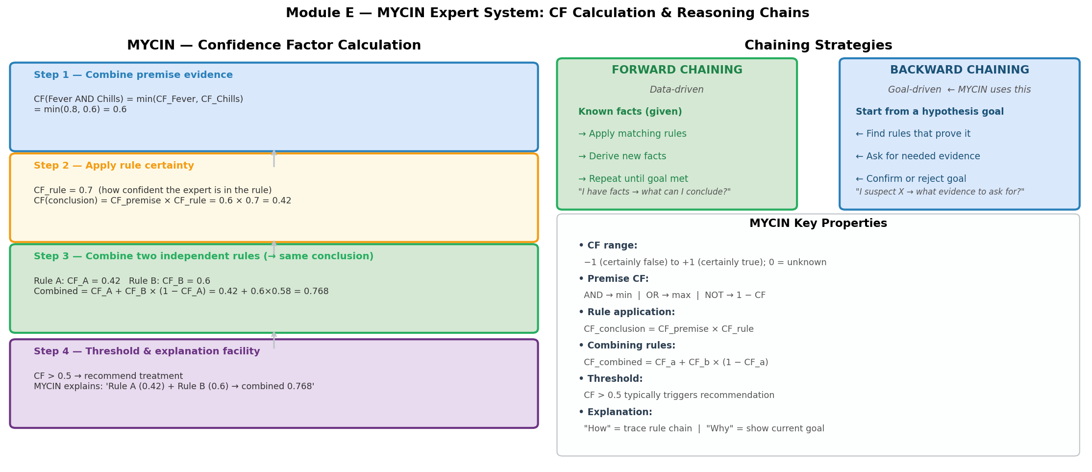
The Junior Doctor with a Giant Manual
Imagine a brand-new doctor on their first day in the hospital. They have zero experience but someone hands them a thick manual – 450 pages of rules written by the best infectious disease specialist in the country. Each page says something like:
“IF the patient’s culture shows gram-negative organisms AND the organism has rod morphology AND the organism is anaerobic, THEN the organism is Bacteroides (I’m about 60% sure).”
The junior doctor doesn’t think creatively. They just follow the manual backwards: they start with a question (“What is causing this infection?”), look up which rules could answer it, then check whether they already know the required facts. If they don’t know something, they either look it up in the patient’s chart or ask the patient directly.
That’s MYCIN. It’s not intelligent in the human sense – it’s a systematic rule-follower with a clever strategy for deciding what to ask.
The Manual is Written in a Weird Language
MYCIN was built in LISP – a programming language where everything is written in prefix notation(前缀表示法)with lots of parentheses:
;; Instead of 2 + 3, you write:
(+ 2 3)          ; → 5

;; Key LISP operations MYCIN uses:
(cons 'a '(b c)) ; → (a b c)   -- prepend an element to a list
(list 'a 'b 'c)  ; → (a b c)   -- create a list
(setq x 5)       ; → x is now 5 -- assign a value to a variable
(eval '(+ 2 3))  ; → 5         -- evaluate an expression
You don’t need to write LISP for the exam, but you should know MYCIN was implemented in LISP and understand prefix notation if given an example.
How Does the Junior Doctor Actually Work?
Let’s walk through a tiny example. Suppose MYCIN’s knowledge base has just three rules:
Rule 1: IF infection is primary-bacteremia
        AND culture-site is sterile-site
        THEN organism is E.coli  (CF = 0.8)

Rule 2: IF organism is E.coli
        THEN recommend drug Ampicillin  (CF = 0.9)

Rule 3: IF infection is primary-bacteremia
        AND patient-age > 60
        THEN organism is Klebsiella  (CF = 0.6)
Goal: “What drug should I recommend?”
Step 1 – MYCIN looks for rules whose THEN part mentions a drug recommendation. It finds Rule 2 (recommend Ampicillin if E.coli). But Rule 2 needs to know the organism. Is it E.coli? Unknown. So “organism is E.coli” becomes a sub-goal.
Step 2 – Now MYCIN searches for rules whose THEN part concludes about the organism. It finds Rule 1. Rule 1 needs two things: (a) infection type and (b) culture site. MYCIN checks working memory (MONITOR). If unknown, it asks the clinician (FINDOUT): “What is the infection type?” The doctor answers: “primary-bacteremia (CF = 1.0).” “What is the culture site?” Answer: “sterile-site (CF = 0.9).”
Step 3 – Now Rule 1 can fire:
- CF(premise) = min(1.0, 0.9) = 0.9 (because AND takes the minimum)
- CF(E.coli) = 0.9 x 0.8 = 0.72
Step 4 – Rule 2 can now fire:
- CF(Ampicillin) = 0.72 x 0.9 = 0.648
MYCIN would report: “I recommend Ampicillin with confidence 0.648.”
This is backward chaining – we started from the goal and worked backwards through the rule chain, only asking questions that were actually needed.
When Does MYCIN Give Up?
MYCIN is smart about not wasting time. It abandons a hypothesis when CF drops below 0.2. Here’s a concrete example of CF propagation down a chain:
Starting hypothesis CF = 0.5
  → Apply Rule (CF_rule = 0.6):
    CF(condition1) = 0.5 x 0.6 = 0.30     (still above 0.2, keep going)
  → Apply next Rule (CF_rule = 0.6):
    CF(condition2) = 0.30 x 0.6 = 0.18    (below 0.2 → ABANDON this path!)
This is efficient: rather than chasing every possible chain of reasoning, MYCIN prunes away paths where confidence has become too low to be useful.
What if Two Rules Support the Same Conclusion?
Suppose Rule 1 gives CF(E.coli) = 0.72 and another Rule 4 also concludes E.coli with CF = 0.5. We combine them:
$$CF_{combined} = 0.72 + 0.5 \times (1 - 0.72) = 0.72 + 0.14 = 0.86$$
Two independent pieces of evidence reinforce each other. Notice the combined CF is higher than either alone, but never reaches 1.0 from two uncertain pieces – that makes intuitive sense!
⚠️ Common Misconception 1: Students often multiply CFs when combining multiple rules for the same conclusion. That’s WRONG. Multiplication is for chaining rules in sequence (premise CF x rule CF). The special combination formula $CF_1 + CF_2(1 - CF_1)$ is for when two different rules both support the same conclusion.
⚠️ Common Misconception 2: Students confuse AND (take the minimum) with OR (take the maximum). Think of it this way – a chain is only as strong as its weakest link (AND = min), but you only need one good reason (OR = max).
⚠️ Common Misconception 3: “IF A THEN B” does NOT mean A is the only cause of B. Multiple rules can conclude B from different premises. Backward chaining identifies possible necessary conditions, not unique ones.
💡 Core Intuition: MYCIN is a backward-chaining rule system that asks only necessary questions, propagates uncertainty through confidence factors, and abandons low-confidence paths early.
📐 正式定义(Formal Definition)
MYCIN Architecture – Three Subprograms
┌─────────────────────────────────────────────────────────────────┐
│                         MYCIN System                            │
│                                                                 │
│  ┌──────────────────────┐    ┌───────────────────────────────┐  │
│  │   Knowledge Base      │    │      Dynamic Data             │  │
│  │   (Persistent,        │    │  (Working Memory,             │  │
│  │    Long-term Memory)  │    │   Per-case, Short-term)       │  │
│  │   450+ IF-THEN rules  │    │   Patient facts gathered      │  │
│  │   with CF values      │    │   during this consultation    │  │
│  └──────────┬────────────┘    └──────────────┬────────────────┘  │
│             │                                │                  │
│  ┌──────────┴────────────────────────────────┴────────────────┐ │
│  │            Inference Engine (MONITOR + FINDOUT)             │ │
│  │            Backward Chaining Controller                    │ │
│  │            Abandons paths when CF < 0.2                    │ │
│  └──────────────────────┬─────────────────────────────────────┘ │
│                         │                                       │
│  ┌──────────────────────┴─────────────────────────────────────┐ │
│  │                                                            │ │
│  │  Subprogram 1:           Subprogram 2:                     │ │
│  │  CONSULTATION SYSTEM     EXPLANATION SYSTEM                │ │
│  │  (Conducts the           (Handles WHY and HOW              │ │
│  │   diagnostic dialogue)    queries from clinician)          │ │
│  │                                                            │ │
│  │  Subprogram 3:                                             │ │
│  │  RULE-ACQUISITION SYSTEM                                   │ │
│  │  (Allows experts to add/modify rules in KB)                │ │
│  │                                                            │ │
│  └────────────────────────────────────────────────────────────┘ │
│                                                                 │
│  ┌────────────────────────────────────────────────────────────┐ │
│  │              User Interface (CLI)                          │ │
│  │  Clinician answers questions, asks WHY/HOW,                │ │
│  │  receives diagnosis and treatment recommendation           │ │
│  └────────────────────────────────────────────────────────────┘ │
└─────────────────────────────────────────────────────────────────┘
Key architectural insight: The separation of Knowledge Base from Inference Engine is what enabled E-MYCIN – remove the medical rules and you get a reusable shell.
Production Rule Format
IF   [condition₁] AND [condition₂] AND ...
THEN [conclusion] WITH CF [confidence_factor]
Concrete example from lecture:
IF   the gram stain of the organism is gram-negative     (condition 1)
AND  the morphology of the organism is rod               (condition 2)
AND  the aerobicity of the organism is anaerobic         (condition 3)
THEN the identity of the organism is Bacteroides  (CF = 0.6)
CF calculation for this rule:
$$CF(\text{conclusion}) = CF(\text{premise}) \times CF(\text{rule})$$
$$CF(\text{premise}) = \min(CF(\text{gram-negative}),; CF(\text{rod}),; CF(\text{anaerobic}))$$
Confidence Factor (CF) Formulas
Range: $CF \in [-1.0, +1.0]$
| Value | Meaning |
|---|---|
| $+1.0$ | Definitely true |
| $+0.7$ | Fairly confident |
| $0.0$ | No information (unknown) |
| $-0.7$ | Fairly confident it’s false |
| $-1.0$ | Definitely false |
Formula 1 – Conjunction (AND) of premises:
$$CF(A \text{ AND } B) = \min(CF_A, ; CF_B)$$
Intuition: a chain is only as strong as its weakest link.
Formula 2 – Disjunction (OR) of premises:
$$CF(A \text{ OR } B) = \max(CF_A, ; CF_B)$$
Intuition: you only need one good reason to believe.
Formula 3 – Rule application (premise → conclusion):
$$CF(\text{conclusion}) = CF(\text{premise}) \times CF(\text{rule})$$
Intuition: uncertainty compounds when you reason through a rule.
Formula 4 – Combining multiple rules for the same conclusion (both positive):
$$CF_{combined} = CF_1 + CF_2 \times (1 - CF_1)$$
Intuition: independent evidence reinforces belief, but with diminishing returns.
Formula 4b – Both negative:
$$CF_{combined} = CF_1 + CF_2 \times (1 + CF_1)$$
Formula 4c – One positive, one negative:
$$CF_{combined} = \frac{CF_1 + CF_2}{1 - \min(|CF_1|, |CF_2|)}$$
For the exam, the “both positive” case (Formula 4) is by far the most commonly tested.
🔄 机制与推导(How It Works)
Forward Chaining vs Backward Chaining – Formal Definitions
Forward Chaining (Data-Driven, A → B)
- Starts from known facts in working memory
- Applies all matching rules to derive new conclusions
- Uses Modus Ponens: IF A is true AND (A → B), THEN B is true
- Direction: facts → conclusions
- Example: “Patient has fever and cough → apply matching rules → conclude possible flu”
Backward Chaining (Goal-Driven, B → A)
- Starts from a hypothesis or goal
- Finds rules whose conclusion matches the goal
- Checks if premises are supported; if not, makes them sub-goals or asks the user
- Direction: hypothesis → required evidence
Critical Logical Distinction (Exam-Critical!)
IF A THEN B means:
  - A is SUFFICIENT for B (A being true is enough to conclude B)
  - B is NECESSARY for A (if B is false, A cannot lead to B)

IMPORTANT: IF A THEN B does NOT mean:
  - A is the ONLY cause of B (other rules may also conclude B!)
  - B implies A (that would be the converse fallacy)

Backward chaining implication:
  - When working backward from B, we find A as a POSSIBLE condition
  - A is a possible necessary condition, but NOT necessarily the unique one
  - Multiple rules can have B as their conclusion
Example: Rule 1 says “IF flu THEN fever.” Rule 2 says “IF meningitis THEN fever.” Starting from “fever” and working backward, we find BOTH flu and meningitis as possible causes – backward chaining identifies possible necessary conditions, not unique ones.
Backward Chaining in MYCIN – Step by Step
GOAL: Determine the identity of the organism

Step 1: Find rules whose THEN mentions "organism identity"
        → Rule 1, Rule 3 are candidates
        → Start with the HIGHEST-CONFIDENCE goal

Step 2: Try Rule 1:
        IF infection = primary-bacteremia  [Unknown → FINDOUT]
        AND site = sterile-site            [Unknown → FINDOUT]
        THEN organism = E.coli (CF=0.8)

Step 3: FINDOUT "infection type" → Clinician answers:
        "primary-bacteremia" (CF = 1.0) → store in Working Memory

Step 4: FINDOUT "culture site" → Clinician answers:
        "sterile-site" (CF = 0.9) → store in Working Memory

Step 5: Rule 1 fires:
        CF(premise) = min(1.0, 0.9) = 0.9
        CF(E.coli)  = 0.9 × 0.8 = 0.72

Step 6: Try Rule 3:
        IF infection = primary-bacteremia  [MONITOR: already known, CF=1.0]
        AND patient-age > 60              [Unknown → FINDOUT]
        THEN organism = Klebsiella (CF=0.6)

Step 7: FINDOUT "patient age" → Clinician answers:
        "age = 72" (CF = 1.0)

Step 8: Rule 3 fires:
        CF(premise) = min(1.0, 1.0) = 1.0
        CF(Klebsiella) = 1.0 × 0.6 = 0.6

Result: E.coli (CF=0.72) vs Klebsiella (CF=0.6)
        → Most likely: E.coli
Notice how MYCIN only asked three questions (infection type, culture site, patient age) – it didn’t ask about every possible fact. That’s the efficiency of backward chaining: ask only what you need.
CF Abandonment Threshold (CF < 0.2)
MYCIN does not chase every hypothesis indefinitely. When a chain of reasoning produces a CF below 0.2, the system abandons that path:
Example: Investigating whether organism X causes the infection

Step 1: Start with hypothesis CF = 0.5
Step 2: Apply Rule (CF_rule = 0.6):
        CF(condition1) = 0.5 × 0.6 = 0.30   ← still ≥ 0.2, continue
Step 3: Apply next Rule (CF_rule = 0.6):
        CF(condition2) = 0.30 × 0.6 = 0.18  ← below 0.2, ABANDON!

The system stops pursuing this line of reasoning because
the accumulated confidence is too low to be useful.
This prevents wasting time on weak hypotheses and focuses the system on the most promising diagnoses.
MONITOR vs FINDOUT – Three-Step Priority
Evaluate premise P:
  1. MONITOR: Is P already in Working Memory?
     → YES: use it (with its associated CF)
     → NO: go to step 2

  2. Are there rules whose conclusion matches P?
     → YES: set P as a sub-goal, recurse (backward chain again)
     → NO: go to step 3

  3. FINDOUT: Ask the user directly
     → Store answer in Working Memory for future MONITOR calls
This three-step priority is crucial: MYCIN avoids redundant questions by always checking memory first.
CF Calculation – Full Worked Example
Scenario: Diagnosing measles with two supporting rules.
Rule A: IF fever(CF=0.8) AND rash(CF=0.6)
        THEN measles (CF_rule = 0.7)

Rule B: IF recent-contact-with-measles-patient(CF=0.9)
        THEN measles (CF_rule = 0.5)
Step 1 – Rule A fires:
$$CF_A(\text{premise}) = \min(0.8, 0.6) = 0.6$$
$$CF_A(\text{measles}) = 0.6 \times 0.7 = 0.42$$
Step 2 – Rule B fires:
$$CF_B(\text{premise}) = 0.9$$
$$CF_B(\text{measles}) = 0.9 \times 0.5 = 0.45$$
Step 3 – Combine Rule A and Rule B (both positive):
$$CF_{combined} = CF_A + CF_B \times (1 - CF_A)$$ $$CF_{combined} = 0.42 + 0.45 \times (1 - 0.42)$$ $$CF_{combined} = 0.42 + 0.45 \times 0.58$$ $$CF_{combined} = 0.42 + 0.261 = 0.681$$
Result: measles with CF = 0.681
Key insight: neither rule alone gives high confidence (0.42 and 0.45), but together they push it to 0.681. Independent evidence accumulates, but never blindly – the formula ensures we can’t exceed 1.0.
Three More Rules – Extended Example
What if a third rule also supports measles with CF = 0.3?
$$CF_{new} = 0.681 + 0.3 \times (1 - 0.681) = 0.681 + 0.3 \times 0.319 = 0.681 + 0.0957 = 0.777$$
Each additional piece of evidence adds less and less – diminishing returns, just like in real life.
Explanation Facility
WHY Query (backward chaining style – “why are you asking this?”):
Clinician: WHY?
MYCIN:     I am trying to determine whether the patient has measles.
           Rule A states:
             IF the patient has fever
             AND the patient has a rash
             THEN there is evidence (CF=0.7) that the diagnosis is measles.
           I already know the patient has fever (CF=0.8).
           I need to know about rash to evaluate this rule.
The WHY query reveals the current backward chaining goal – it shows which rule MYCIN is trying to evaluate and why it needs the requested information.
HOW Query (forward chaining style – “how did you conclude that?”):
Clinician: HOW measles?
MYCIN:     I used Rule A and Rule B.
           Rule A concluded measles (CF=0.42) based on:
             - fever (CF=0.8) [told by clinician]
             - rash (CF=0.6) [told by clinician]
           Rule B concluded measles (CF=0.45) based on:
             - recent contact with measles patient (CF=0.9) [told by clinician]
           Combined CF = 0.681
The HOW query traces the forward chain of reasoning that led to the conclusion – it shows which rules fired and what evidence was used.
This transparency is a major advantage of rule-based systems over modern neural networks.
⚖️ 权衡分析(Trade-offs & Comparisons)
Forward Chaining vs Backward Chaining
| Aspect | Forward Chaining(前向链接) | Backward Chaining(后向链接) |
|---|---|---|
| Direction | Facts → Conclusions (A → B) | Goal → Required Evidence (B → A) |
| Logical basis | Modus Ponens | Hypothesis testing |
| Analogy | A scientist observing data and forming theories | A detective testing a hypothesis |
| Starting point | Known facts in working memory | A specific goal or hypothesis |
| Question strategy | Doesn’t ask questions – uses what’s available | Asks targeted questions to fill gaps |
| Efficiency | May explore many irrelevant rules | Focused – only explores rules relevant to the goal |
| Best for | Monitoring, alerting, configuration | Diagnosis, planning, troubleshooting |
| MYCIN uses | No (not primary) | Yes (primary inference method) |
| Sufficiency | A is SUFFICIENT for B | B is NECESSARY for A |
| Risk | Combinatorial explosion of derived facts | Deep recursion if rule chains are long |
A is SUFFICIENT for B vs B is NECESSARY for A
Rule: IF A THEN B

Forward (A → B):
  "If I have A, that is SUFFICIENT to conclude B."
  "A is enough. Having A guarantees B."

Backward (B → A):
  "If I want B, then A is a NECESSARY condition."
  "I need A (among possibly other things) to get B."

BUT: A is NOT the ONLY way to get B!
     Other rules may also conclude B from different premises.
     Backward chaining finds POSSIBLE necessary conditions.
Expert Systems vs Modern Machine Learning
| Feature | Expert System (MYCIN) | Machine Learning (e.g., Neural Network) |
|---|---|---|
| Knowledge source | Human experts (manual encoding) | Data (automated learning) |
| Knowledge form | Explicit IF-THEN rules | Implicit weights in a model |
| Explainability | High – can trace every rule (WHY/HOW) | Low – often a “black box” |
| Learning | None – rules are fixed | Yes – improves with more data |
| Handling uncertainty | Confidence Factors (handcrafted) | Probabilistic outputs (learned) |
| Coverage | Only what rules cover (brittle) | Can generalise to unseen cases |
| Domain transfer | E-MYCIN shell (but needs new rules) | Transfer learning, fine-tuning |
| Maintenance | Hard – manually update rules | Retrain on new data |
| Data requirement | Needs experts, not data | Needs large datasets, not experts |
MYCIN vs Bayesian Networks
| Feature | MYCIN (CF) | Bayesian Network |
|---|---|---|
| Theoretical basis | Ad hoc (not formally probabilistic) | Probability theory (rigorous) |
| Independence assumption | Rules are somewhat independent | Models dependencies explicitly |
| Combination formula | $CF_1 + CF_2(1 - CF_1)$ | Bayes’ theorem with priors |
| Ease of use | Simple for experts to assign CFs | Requires conditional probabilities |
| Accuracy | Good enough in practice | Theoretically more sound |
🏗️ 设计题答题框架
If asked: “Explain backward chaining for medical diagnosis” (S1 2025 Sample Q6 style)
WHAT: “Backward chaining is a goal-driven reasoning strategy used in expert systems like MYCIN. It starts with a hypothesis (e.g., a possible diagnosis) and works backward through the rule base to find supporting evidence in the patient’s symptoms.”
WHY: “Backward chaining is more efficient than forward chaining for diagnosis because it only asks the clinician for information that is actually needed to evaluate relevant rules, rather than gathering all possible data first.”
HOW: “The inference engine sets a top-level goal (e.g., ‘what is the diagnosis?’). It finds rules whose THEN part matches the goal. For each rule, it checks whether the IF conditions are known (MONITOR). If not, conditions become sub-goals, recursively applying the same process. If no rule can derive a fact, the system uses FINDOUT to ask the clinician. The system starts with the highest-confidence goal and abandons paths when CF drops below 0.2.”
TRADE-OFF: “The advantage is efficiency and transparency (the WHY/HOW facility lets clinicians understand the reasoning). The limitation is the knowledge acquisition bottleneck – all 450+ rules had to be manually encoded by interviewing domain experts.”
EXAMPLE: “To determine the organism: MYCIN finds Rule 1 (IF infection=bacteremia AND site=sterile THEN E.coli CF=0.8). It asks for infection type and culture site, then computes CF(E.coli) = min(1.0, 0.9) x 0.8 = 0.72.”
If asked: “Calculate the combined CF” (computation question)
Step 1: For each rule, compute CF(premise) using AND = min, OR = max.
Step 2: Compute CF(conclusion) = CF(premise) x CF(rule) for each rule.
Step 3: If multiple rules support the same conclusion, combine: $CF_{combined} = CF_1 + CF_2(1 - CF_1)$.
Step 4: State the final CF value and interpret it (e.g., “moderately confident”).
If asked: “What is E-MYCIN and why is it significant?”
WHAT: “E-MYCIN (Essential MYCIN) is the first domain-independent expert system shell, created by removing MYCIN’s medical knowledge base while retaining the inference engine, explanation facility, and user interface.”
WHY: “It demonstrated that the reasoning architecture could be separated from domain knowledge, making it reusable across fields.”
HOW: “To build a new expert system, developers load a new knowledge base into the E-MYCIN shell. The backward chaining engine, CF propagation, and WHY/HOW facilities work unchanged.”
EXAMPLE: “E-MYCIN was used to build SACON (structural engineering analysis) and PUFF (pulmonary function diagnosis) – different domains, same inference engine.”
LIMITATION: “While the shell is reusable, encoding new domain knowledge still requires extensive expert interviews – the knowledge acquisition bottleneck remains.”
📝 历年真题与考试练习(Exam Questions & Practice)
S1 2025 Sample Q6 (3 marks) – Backward Chaining for Medical Diagnosis
Question: Explain how backward chaining works for medical diagnosis. Use the following scenario: A patient has a runny nose. Possible diagnoses include common cold, allergies, and measles.
Click to reveal model answer
Backward chaining is goal-driven reasoning. We start with hypotheses (possible diagnoses) and work backward to find supporting evidence in the patient’s symptoms.
Step 1 – List hypotheses to test:
- Hypothesis 1: Common Cold
- Hypothesis 2: Allergies
- Hypothesis 3: Measles
Step 2 – Test each hypothesis by checking required symptoms:
Support “Common Cold”:
- Rule: IF runny nose AND sore throat AND mild fever THEN common cold (CF=0.7)
- Runny nose? YES (given) ✓
- Sore throat? Need to check → FINDOUT
- Mild fever? Need to check → FINDOUT
Support “Allergies”:
- Rule: IF runny nose AND history of allergies AND itchy eyes THEN allergies (CF=0.6)
- Runny nose? YES (given) ✓
- History of allergies? Need to check → FINDOUT
- Itchy eyes? Need to check → FINDOUT
Support “Measles”:
- Rule: IF runny nose AND distinctive rash AND high fever THEN measles (CF=0.8)
- Runny nose? YES (given) ✓
- Distinctive rash? Need to check → FINDOUT
- High fever? Need to check → FINDOUT
Step 3 – System asks targeted questions based on which hypotheses it is testing. It does NOT ask about every possible symptom – only those needed to evaluate the current rules.
Step 4 – Calculate CFs for each hypothesis based on evidence gathered, and report the diagnosis with the highest combined CF.
Key points for marks:
- Start from hypothesis, not from data (1 mark)
- Only ask questions needed to evaluate relevant rules (1 mark)
- Show specific example of checking symptoms against rules (1 mark)
Practice Question 1 – CF Calculation (8 marks)
Consider the following MYCIN rules:
Rule 1: IF patient-has-fever (CF=0.9)
        AND patient-has-stiff-neck (CF=0.7)
        THEN diagnosis is meningitis (CF_rule = 0.8)

Rule 2: IF patient-has-fever (CF=0.9)
        AND cerebrospinal-fluid-is-cloudy (CF=0.85)
        THEN diagnosis is meningitis (CF_rule = 0.75)
(a) Calculate the CF for meningitis from Rule 1 alone. (3 marks)
(b) Calculate the CF for meningitis from Rule 2 alone. (3 marks)
(c) Calculate the combined CF for meningitis using both rules. (2 marks)
Click to reveal answer
(a) Rule 1:
$$CF_1(\text{premise}) = \min(0.9, 0.7) = 0.7$$ $$CF_1(\text{meningitis}) = 0.7 \times 0.8 = 0.56$$
(b) Rule 2:
$$CF_2(\text{premise}) = \min(0.9, 0.85) = 0.85$$ $$CF_2(\text{meningitis}) = 0.85 \times 0.75 = 0.6375$$
(c) Combined:
$$CF_{combined} = 0.56 + 0.6375 \times (1 - 0.56)$$ $$= 0.56 + 0.6375 \times 0.44$$ $$= 0.56 + 0.2805$$ $$= 0.8405$$
Interpretation: MYCIN would be fairly confident (CF approximately 0.84) that the diagnosis is meningitis.
Practice Question 2 – Forward vs Backward Chaining (6 marks)
Explain the difference between forward chaining and backward chaining in expert systems. Which does MYCIN use and why? Illustrate with a medical diagnosis example.
Click to reveal answer framework
Forward Chaining (2 marks):
- Data-driven: starts with known facts in working memory
- Applies all matching rules to derive new facts via Modus Ponens (IF A is true AND A→B, THEN B)
- Continues until a goal is reached or no more rules fire
- A is sufficient for B
- Example: “Patient has fever and cough → apply rules → conclude possible flu”
Backward Chaining (2 marks):
- Goal-driven: starts with a hypothesis or goal
- Finds rules whose conclusion matches the goal
- Checks if premises are known; if not, creates sub-goals or asks the user
- B is necessary for A (but NOT the only cause!)
- Example: “Is the patient’s infection caused by E.coli? → What evidence do I need? → Ask for infection type and culture site”
Why MYCIN uses backward chaining (2 marks):
- Medical diagnosis is naturally hypothesis-driven
- More efficient: only asks the clinician for information relevant to the current hypothesis
- Avoids gathering unnecessary data (forward chaining might explore hundreds of irrelevant rules)
- Supports the WHY explanation: “I am asking about X because I am trying to determine Y”
- Can abandon low-confidence paths early (CF < 0.2 threshold)
Practice Question 3 – MYCIN Architecture (5 marks)
Draw and label the main components of the MYCIN expert system. Explain the role of each component.
Click to reveal answer framework
Components to include:
- Knowledge Base (KB) – 450+ production rules encoding medical expertise (IF-THEN with CF values). This is persistent, long-term memory.
- Dynamic Data / Working Memory – Stores currently known facts about the patient being diagnosed. Per-case, short-term.
- Inference Engine – Applies backward chaining; uses MONITOR (check memory) and FINDOUT (ask user). Starts with highest-confidence goal, abandons when CF < 0.2.
- Three Subprograms:
- Subprogram 1: Consultation System – conducts the diagnostic dialogue
- Subprogram 2: Explanation System – handles WHY queries (backward style) and HOW queries (forward style)
- Subprogram 3: Rule-Acquisition System – allows experts to add/modify rules
- User Interface – Clinician interacts via Q&A; provides data and can query the system
Key point: The separation of Knowledge Base from Inference Engine enabled E-MYCIN – the first expert system shell. Remove the medical rules and the inference engine can be reused for other domains.
Practice Question 4 – Tracing a Backward Chain (7 marks)
Given the following rules:
Rule 1: IF A AND B THEN C (CF=0.9)
Rule 2: IF C AND D THEN E (CF=0.8)
Rule 3: IF A AND F THEN C (CF=0.7)
Facts in working memory: A (CF=1.0), B (CF=0.8), D (CF=0.7), F (CF=0.6)
Goal: Determine E.
(a) Trace the backward chaining process. (3 marks)
(b) Calculate the final CF of E, accounting for Rules 1 and 3 both concluding C. (4 marks)
Click to reveal answer
(a) Backward chaining trace:
- Goal = E. Find rules with E in conclusion → Rule 2: IF C AND D THEN E
- Check C: Unknown → sub-goal. Check D: Known (CF=0.7) via MONITOR.
- Sub-goal = C. Find rules with C in conclusion → Rule 1 and Rule 3.
- Rule 1: Need A (known, CF=1.0) and B (known, CF=0.8). Both available via MONITOR.
- Rule 3: Need A (known, CF=1.0) and F (known, CF=0.6). Both available via MONITOR.
- No FINDOUT needed – all facts are in working memory.
(b) CF Calculation:
Rule 1 → C: $$CF_1(\text{premise}) = \min(1.0, 0.8) = 0.8$$ $$CF_1(C) = 0.8 \times 0.9 = 0.72$$
Rule 3 → C: $$CF_3(\text{premise}) = \min(1.0, 0.6) = 0.6$$ $$CF_3(C) = 0.6 \times 0.7 = 0.42$$
Combine Rule 1 and Rule 3 for C: $$CF(C) = 0.72 + 0.42 \times (1 - 0.72) = 0.72 + 0.42 \times 0.28 = 0.72 + 0.1176 = 0.8376$$
Now Rule 2 → E: $$CF_2(\text{premise}) = \min(CF(C), CF(D)) = \min(0.8376, 0.7) = 0.7$$ $$CF(E) = 0.7 \times 0.8 = 0.56$$
Final answer: CF(E) = 0.56
Practice Question 5 – Quick CF Drill (3 marks)
Rule X: IF P(CF=0.7) AND Q(CF=0.5) THEN R (CF=0.6). What is CF(R)?
Click to reveal answer
$$CF(\text{premise}) = \min(0.7, 0.5) = 0.5$$ $$CF(R) = 0.5 \times 0.6 = 0.30$$
Practice Question 6 – CF Abandonment (2 marks)
A backward chaining path starts with hypothesis CF=0.5. Each subsequent rule in the chain has CF_rule=0.6. After how many rule applications does MYCIN abandon this path (threshold: CF < 0.2)?
Click to reveal answer
$$\text{After Rule 1: } CF = 0.5 \times 0.6 = 0.30 \quad (\geq 0.2, \text{ continue})$$ $$\text{After Rule 2: } CF = 0.30 \times 0.6 = 0.18 \quad (< 0.2, \text{ ABANDON})$$
Answer: After 2 rule applications, the CF drops to 0.18 which is below the 0.2 threshold, so MYCIN abandons this path.
Practice Question 7 – WHY and HOW Queries (3 marks)
Explain what information the WHY and HOW queries reveal in MYCIN. Which type of chaining does each correspond to?
Click to reveal answer
WHY query (1.5 marks):
- Corresponds to backward chaining style
- Reveals the system’s current reasoning goal
- When MYCIN asks “What is the patient’s temperature?” and the clinician responds “WHY?”, MYCIN explains: “I am trying to determine if the patient has meningitis. Rule 5 states IF fever AND stiff neck THEN meningitis. I need to know about fever to evaluate this rule.”
- Shows the chain of reasoning from goal to current question
HOW query (1.5 marks):
- Corresponds to forward chaining style
- Shows the rule chain that led to a specific conclusion
- When the clinician asks “HOW did you conclude meningitis?”, MYCIN traces forward through the rules it used and the evidence it gathered
- Shows: “I used Rule 5 (fever=yes, CF=0.9 AND stiff neck=yes, CF=0.7) to conclude meningitis with CF=0.56”
🌐 英语表达要点(English Expression)
Describing MYCIN’s Architecture
"MYCIN is a rule-based expert system developed by Ted Shortliffe at Stanford
 in the 1970s. It consists of a knowledge base containing over 450 production
 rules, dynamic working memory for patient data, and an inference engine that
 performs backward chaining. It has three main subprograms: a consultation
 system, an explanation system, and a rule-acquisition system."
Explaining Backward Chaining
"Backward chaining is a goal-driven reasoning strategy. The system begins
 with a diagnostic goal, identifies rules whose conclusions match that goal,
 and then evaluates the premises. If a premise is unknown, it becomes a
 sub-goal, and the process recurses until all required facts are determined.
 The system starts with the highest-confidence goal and abandons paths when
 confidence drops below 0.2."
Explaining the Sufficient/Necessary Distinction
"In the rule IF A THEN B, A is sufficient for B — having A is enough to
 conclude B. Conversely, B is necessary for A — if B is false, A cannot
 lead to B through this rule. However, A is not the only cause of B;
 other rules may also conclude B from different premises."
Explaining CF Calculation
"The confidence factor for a conjunctive premise is the minimum of the
 individual CFs. The conclusion CF is then computed by multiplying the
 premise CF by the rule's CF. When multiple rules support the same
 conclusion, they are combined using the formula CF₁ + CF₂(1 - CF₁)."
Explaining E-MYCIN
"E-MYCIN is the first domain-independent expert system shell, derived from
 MYCIN. By separating the inference engine from the medical knowledge base,
 the architecture became reusable for building expert systems in other
 domains such as structural engineering (SACON) and pulmonary function
 diagnosis (PUFF)."
易错表达 / Common Mistakes in English
| Incorrect | Correct |
|---|---|
| “MYCIN uses forward chaining” | “MYCIN uses backward chaining (goal-driven)” |
| “CFs are probabilities” | “CFs are not probabilities; they range from -1 to +1 and use different combination rules” |
| “Multiply CFs to combine two rules” | “Multiply for rule application (premise x rule CF); use the combination formula for two rules supporting the same conclusion” |
| “MYCIN learns from experience” | “MYCIN does not learn; its rules are manually encoded and remain fixed” |
| “E-MYCIN is a different expert system” | “E-MYCIN is a domain-independent shell – the same inference engine without domain-specific rules” |
| “IF A THEN B means A is the only cause of B” | “IF A THEN B means A is sufficient for B, but other rules can also conclude B” |
| “Backward chaining finds THE necessary condition” | “Backward chaining finds possible necessary conditions (not unique ones)” |
关键词汇
- backward chaining (not “backward chained” when used as a noun/modifier)
- confidence factor (not “confidence level” or “certainty factor” – stick with “confidence factor” for MYCIN)
- production rule (not “production” alone)
- knowledge acquisition bottleneck (the standard term for the core limitation)
- domain-independent shell (the correct description of E-MYCIN)
- Modus Ponens (the logical basis for forward chaining: IF A AND A→B THEN B)
- prefix notation (LISP’s way of writing expressions, e.g., (+ 2 3) instead of 2+3)
🔧 Practical Applications (Modern Relevance)
While MYCIN itself was never deployed clinically, its ideas live on in modern business rules engines:
| System | Description |
|---|---|
| Drools (Java) | Open-source business rules engine; uses forward and backward chaining on production rules |
| Nools (JavaScript) | Rules engine for Node.js, inspired by Drools |
| CLIPS | C-based expert system tool descended from NASA’s work |
These systems are used today for fraud detection, insurance claim processing, medical decision support, and compliance checking – essentially any domain where decisions can be encoded as IF-THEN rules with certainty measures.
🔬 Evaluation of MYCIN
- Expert panel comparison: MYCIN’s diagnoses were compared against those of Stanford infectious disease specialists
- Result: MYCIN achieved approximately 65% correct diagnoses, comparable to the specialists on the panel
- Key finding: High agreement between MYCIN’s recommendations and expert consensus
- However: MYCIN was never deployed clinically due to legal, ethical, and practical concerns (Who is liable if the system is wrong? Clinicians didn’t trust a computer system in the 1970s)
- Legacy: Demonstrated that expert systems could perform at expert level in narrow domains; led to the expert systems boom of the 1980s
✅ 自测检查清单
- 能画出 MYCIN 的架构图并标注 KB, Working Memory, Inference Engine, 三个子程序 (Consultation, Explanation, Rule-Acquisition)?
- 能用英文解释 backward chaining 的完整流程(Goal → Find rules → Check premises → Sub-goal/FINDOUT → Recurse)?
- 能区分 MONITOR 和 FINDOUT 的作用?
- 能正确计算 CF(AND) = min, CF(OR) = max?
- 能正确计算 CF(conclusion) = CF(premise) x CF(rule)?
- 能正确使用组合公式 CF_combined = CF_1 + CF_2(1 - CF_1)?
- 能在一道多规则题目中完成完整的 CF 计算链?
- 能解释 WHY(backward style)和 HOW(forward style)查询分别揭示什么?
- 能解释 E-MYCIN 的意义(第一个领域无关的推理外壳)?
- 能列出 MYCIN 的局限性(knowledge acquisition bottleneck, brittleness, no learning)?
- 能对比 Forward Chaining vs Backward Chaining 并解释 sufficient vs necessary?
- 能解释 “IF A THEN B” 不代表 A 是 B 的唯一原因?
- 知道 MYCIN 在 CF < 0.2 时放弃假设?
- 知道 MYCIN 的评估结果(65% correct, comparable to specialists, never deployed clinically)?
- 知道 LISP 的前缀表示法 (prefix notation)?
- 能用 backward chaining 分析一个医学诊断场景(如 S1 2025 Q6 的 runny nose 例子)?
Decision Trees & Ensemble Methods (Week 4 Lecture 2)
🎯 Exam Importance
🔴 必考 | Sample Test Q5 (3 marks), Actual S1 2025 Q4 (2 marks), S1 2026 Sample Q5 (3 marks)
Random Forest feature bagging is directly tested in Q5. CART’s greedy nature is tested in Q4. Entropy, Information Gain, and the Bagging vs Boosting distinction are foundational concepts that appear across multiple question types. You must be able to calculate entropy, explain why feature bagging decorrelates trees, explain what “greedy” means for CART, and trace through an AdaBoost round with numbers.
📖 Core Concepts
| English Term | 中文 | One-line Definition |
|---|---|---|
| Decision Tree(决策树) | 决策树 | A tree-structured classifier: internal nodes test features, branches represent values, leaves assign class labels |
| Root Node(根节点) | 根节点 | The topmost node that represents the first split on the entire dataset |
| Internal / Decision Node(内部节点) | 内部节点 / 决策节点 | A non-leaf node that tests a feature and branches based on the result |
| Leaf Node(叶节点) | 叶节点 | A terminal node that assigns a class label (classification) or value (regression) |
| Classification Tree(分类树) | 分类树 | Discrete output; leaf assigns majority class of the samples reaching it |
| Regression Tree(回归树) | 回归树 | Continuous output; leaf assigns mean value of the samples reaching it |
| CART(分类回归树) | 分类回归树 | Classification And Regression Trees – always performs binary splits, uses Gini impurity |
| ID3 | ID3 算法 | Iterative Dichotomiser 3 – multiway splits, categorical features only, uses Information Gain |
| C4.5 | C4.5 算法 | Extension of ID3 – handles continuous features, converts tree to rules, performs pruning |
| Entropy $H(X)$(熵) | 熵 | $H(X) = -\sum p(x) \log_2 p(x)$ – measures impurity/uncertainty in a distribution |
| Joint Entropy $H(X,Y)$(联合熵) | 联合熵 | Uncertainty when considering two variables jointly |
| Specific Conditional Entropy $H(Y|X=x)$ | 特定条件熵 | $H(Y|X=x) = -\sum p(y|x) \log_2 p(y|x)$ – uncertainty about $Y$ given a specific value of $X$ |
| Conditional Entropy $H(Y|X)$(条件熵) | 条件熵 | $H(Y|X) = \sum P(X=x),H(Y|X=x)$ – remaining uncertainty about $Y$ after knowing $X$ |
| Information Gain(信息增益) | 信息增益 | $IG(Y|X) = H(Y) - H(Y|X)$ – how much knowing $X$ reduces uncertainty about $Y$ |
| Gini Impurity(基尼不纯度) | 基尼不纯度 | $\text{Gini}(t) = 1 - \sum p_i^2$ – alternative splitting criterion used in CART |
| Pruning(剪枝) | 剪枝 | Removing subtrees/leaf nodes to reduce overfitting; evaluate effect of deleting leaf nodes |
| Ensemble Method(集成方法) | 集成学习 | Combining multiple weak learners into one strong learner |
| Bagging(自助聚合) | 袋装法 / 自助聚合 | Bootstrap Aggregating – train models independently on bootstrap samples, aggregate by vote/average |
| Bootstrap Sample(自助样本) | 自助样本 | A sample of size $n$ drawn with replacement from a dataset of size $n$ |
| Random Forest(随机森林) | 随机森林 | Bagging + feature bagging: at each split, only $\sqrt{p}$ random features are considered |
| Feature Bagging(特征袋装) | 特征袋装 | Randomly selecting a subset of features at each split to decorrelate trees |
| Boosting(提升法) | 提升法 | Sequential training where each new model focuses on errors of previous ones |
| AdaBoost(自适应提升) | 自适应提升 | Adaptive Boosting – re-weights misclassified samples each round, combines weighted weak learners |
| Gradient Boosting(梯度提升) | 梯度提升 | Each new tree fits the residual errors (negative gradients) of the current ensemble |
| XGBoost(极端梯度提升) | 极端梯度提升 | Optimised gradient boosting with regularisation in the objective |
| Weak Learner(弱学习器) | 弱学习器 | A classifier only slightly better than random chance (e.g., a decision stump) |
| Decision Stump(决策桩) | 决策桩 | A decision tree with exactly one split (depth 1) |
| Bias(偏差) | 偏差 | Systematic error from a model too simple to capture the true relationship |
| Variance(方差) | 方差 | Sensitivity to training data – how much the model changes with different samples |
| NP-complete(NP 完全) | NP 完全问题 | Finding the optimal decision tree is computationally intractable; hence we use greedy heuristics |
🧠 Feynman Draft – Learning From Scratch
The 20 Questions Game
Imagine you are playing the game “20 Questions(20个问题游戏).” Someone thinks of an animal, and you ask yes/no questions to narrow down the answer: “Is it bigger than a cat?” → “Does it live in water?” → “Does it have stripes?” Each question splits the remaining possibilities into two groups, and after enough questions you arrive at the answer.
That is exactly how a decision tree works. Each internal node asks a question about one feature (e.g., “Is income > $50K?”). Each branch is the answer (yes/no). Each leaf is the final prediction (e.g., “will repay loan” or “will default”).
Trees are Surprisingly Powerful
A decision tree can express any Boolean function. Think about it: for any truth table, you can build a tree that tests each input variable along a path from root to leaf. The tree might be huge, but it can always represent the function.
A decision tree can also approximate any continuous function (given enough depth and data).
Even better: every path from root to leaf maps directly to an IF-THEN rule:
Path: [root] Outlook=Sunny → [node] Humidity=High → [leaf] Don't Play

Rule: IF Outlook = Sunny AND Humidity = High THEN Don't Play Tennis
So a decision tree is essentially a set of rules – just organized as a tree for efficient evaluation.
What Makes a Good Question?
Not all questions are equally useful. Asking “Is it alive?” when you already know it is an animal is worthless – it does not split anything. The best question is one that reduces your uncertainty the most.
Entropy measures this uncertainty. Think of it as “how surprised are you, on average, by the outcome?”
- Fair coin flip: You have no idea what is coming – maximum surprise. $H = 1$ bit.
- Biased coin (90% heads): You mostly expect heads – less surprise. $H \approx 0.47$ bits.
- Certain outcome (100% heads): No surprise at all. $H = 0$ bits.
Information Gain tells you how much a particular question reduces entropy. You always pick the question with the highest Information Gain – the one that tells you the most.
But Finding the Best Tree is Impossible…
Here’s the catch: finding the optimal decision tree (the smallest tree that correctly classifies all training data) is an NP-complete problem. That means there’s no known algorithm that can solve it efficiently for large datasets.
So what do we do? We use a greedy heuristic: at each node, pick the best split right now without worrying about future splits. This is fast but not guaranteed to find the global optimum.
Toy Entropy Calculation
Suppose you have 10 emails: 6 spam, 4 not-spam.
$$H(Y) = -\frac{6}{10}\log_2\frac{6}{10} - \frac{4}{10}\log_2\frac{4}{10}$$ $$= -0.6 \times (-0.737) - 0.4 \times (-1.322)$$ $$= 0.442 + 0.529 = 0.971 \text{ bits}$$
Now you split on the feature “contains FREE”:
- “FREE” group: 5 emails (5 spam, 0 not-spam) → $H = 0$ (pure!)
- “no FREE” group: 5 emails (1 spam, 4 not-spam) → $H = -\frac{1}{5}\log_2\frac{1}{5} - \frac{4}{5}\log_2\frac{4}{5} = 0.722$ bits
Conditional entropy after split:
$$H(Y|X) = \frac{5}{10} \times 0 + \frac{5}{10} \times 0.722 = 0.361 \text{ bits}$$
Information Gain: $IG = 0.971 - 0.361 = 0.610$ bits. This is a great split!
From One Tree to a Forest – Wisdom of Crowds
A single decision tree is like asking one person for their opinion. That person might be knowledgeable but also biased – they might latch onto irrelevant quirks of their own experience. This is overfitting: the tree memorises the training data (high variance).
Now imagine asking 2,048 different people, each of whom:
- Studied a slightly different version of the material (different bootstrap samples of data)
- Focused on different aspects (different random subsets of features)
Then you take a majority vote. Individual errors cancel out. This is Random Forest(随机森林) – the “wisdom of crowds” for machine learning.
Why Feature Bagging is Essential (Not Just Data Bagging!)
Here’s a subtle but critical point. Even with bagging (training on different bootstrap samples), if one feature is overwhelmingly strong (say, “blood sugar level” for predicting diabetes), every tree will put that feature at the root. The trees become nearly identical despite seeing different data subsets. Averaging 2,048 identical trees is no better than having one tree.
Feature bagging solves this: at each split, only $\sqrt{p}$ randomly chosen features are considered. Most trees won’t even have the dominant feature available at their root. This forces diversity – trees explore different parts of the feature space and make different kinds of errors, which average out beautifully.
Bagging vs Boosting – Two Strategies for Teamwork
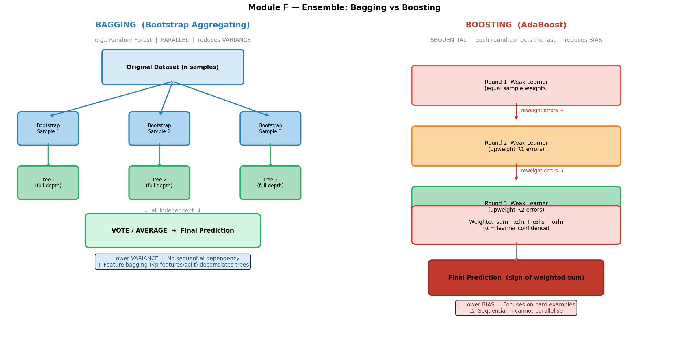
Bagging(袋装法) = “parallel teamwork.” Everyone works independently on their own slightly different version of the problem. Then you average. Good when each individual is smart but unreliable (high variance).
Boosting(提升法) = “sequential coaching.” The first person tries, the second person specifically studies the first person’s mistakes, the third person studies mistakes that remain, and so on. Good when each individual is weak/simple (high bias).
⚠️ Common Misconception 1: Many students confuse feature bagging with data bagging (bootstrapping). They are two separate things that happen together in Random Forest:
- Data bagging = each tree trains on a different bootstrap sample of the data (sample with replacement)
- Feature bagging = at each split, each tree only considers $\sqrt{p}$ randomly chosen features
Both are needed. Data bagging alone is just “Bagging.” Adding feature bagging on top makes it “Random Forest.”
⚠️ Common Misconception 2: Students think “greedy” means “fast” or “lazy.” In decision trees, greedy means the algorithm selects the best split at each node without looking ahead to see how that split affects future nodes. It makes the locally optimal choice, which may not be globally optimal.
⚠️ Common Misconception 3: “Bagging reduces bias” – NO! Bagging reduces variance. Boosting reduces bias.
💡 Core Intuition: Many diverse, slightly-wrong trees vote together to produce one highly accurate prediction – strength through diversity.
📐 Formal Definitions
Entropy(熵)
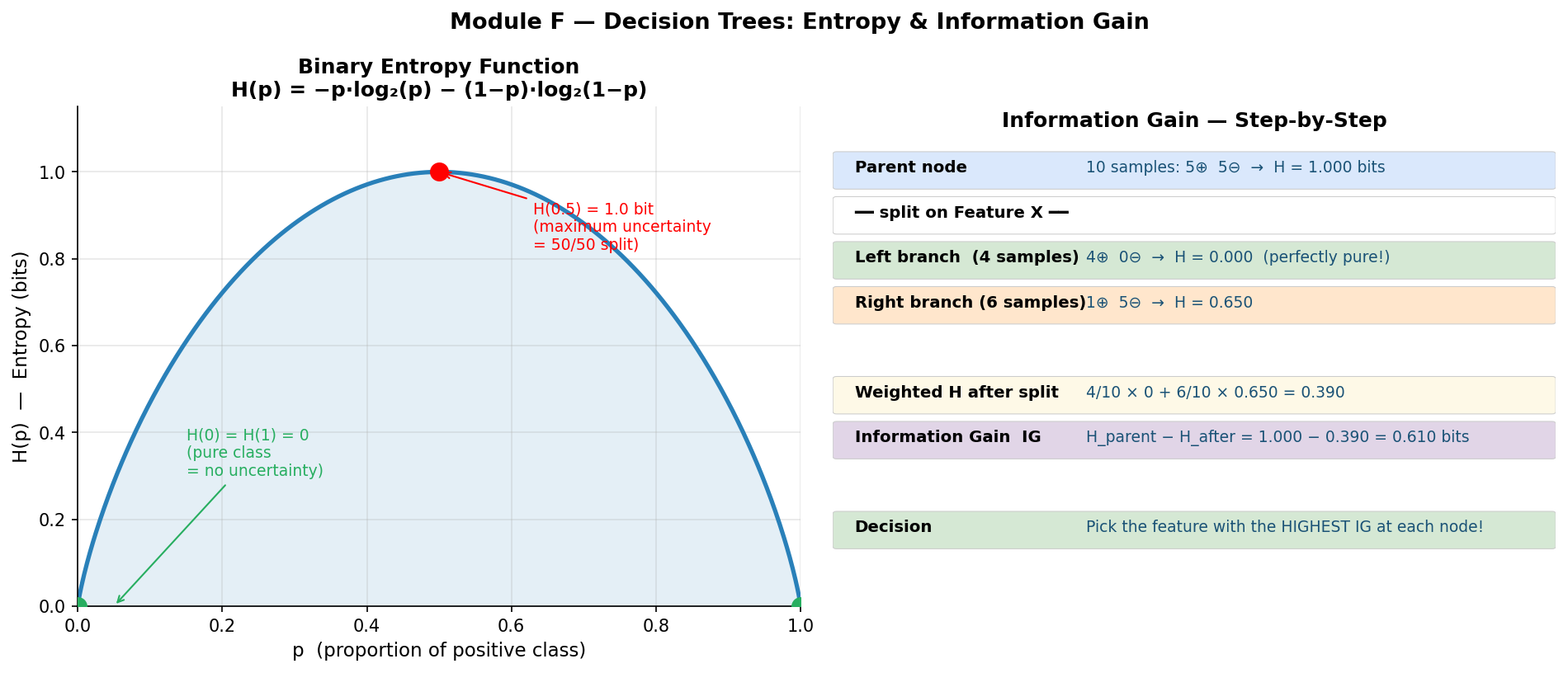
Entropy measures the average uncertainty (impurity) in a probability distribution:
$$H(X) = -\sum_{x \in \mathcal{X}} p(x) \log_2 p(x)$$
Key properties:
- $H(X) \geq 0$ always
- $H(X) = 0$ iff one outcome has probability 1 (complete certainty)
- For binary classification: $H_{\max} = 1$ bit (when $p = 0.5$)
- More classes → higher potential entropy: $H_{\max} = \log_2 k$ for $k$ classes
- Maximum when uniform: for binary case, $p = 0.5$ gives $H = 1$ bit
Canonical examples:
- Fair coin: $H = -0.5\log_2(0.5) - 0.5\log_2(0.5) = 0.5 + 0.5 = 1$ bit
- Biased coin ($p=0.9$): $H = -0.9\log_2(0.9) - 0.1\log_2(0.1) = 0.137 + 0.332 = 0.469$ bits
Joint Entropy(联合熵)
The uncertainty when considering two random variables together:
$$H(X, Y) = -\sum_{x \in \mathcal{X}} \sum_{y \in \mathcal{Y}} p(x, y) \log_2 p(x, y)$$
Specific Conditional Entropy(特定条件熵)
The entropy of $Y$ given a specific value of $X$:
$$H(Y | X = x) = -\sum_{y \in \mathcal{Y}} p(y | x) \log_2 p(y | x)$$
This measures: “How uncertain am I about $Y$ when I know $X$ takes value $x$?”
Conditional Entropy(条件熵)
The expected remaining uncertainty about $Y$ after observing $X$:
$$H(Y | X) = \sum_{x \in \mathcal{X}} P(X = x), H(Y | X = x)$$
This is a weighted average of the specific conditional entropies, weighted by the probability of each value of $X$.
Expanded form:
$$H(Y | X) = -\sum_{x \in \mathcal{X}} \sum_{y \in \mathcal{Y}} p(x, y) \log_2 p(y | x)$$
Entropy Properties (Exam-Critical)
- Non-negativity: $H(X) \geq 0$
- Chain Rule: $H(X, Y) = H(X | Y) + H(Y) = H(Y | X) + H(X)$
- Independence: If $X$ and $Y$ are independent, $H(Y | X) = H(Y)$ (knowing $X$ tells you nothing about $Y$)
- Conditioning reduces entropy: $H(Y | X) \leq H(Y)$ (knowing something never increases uncertainty)
Information Gain(信息增益)
$$IG(Y | X) = H(Y) - H(Y | X)$$
- If $X$ tells us nothing about $Y$: $IG = 0$
- If $X$ perfectly determines $Y$: $IG = H(Y)$ (all uncertainty removed)
- Always non-negative: $IG \geq 0$ (knowing something never increases uncertainty)
Decision tree splitting rule: At each node, choose the feature $X^$ that maximises $IG(Y | X^)$.
Gini Impurity(基尼不纯度)– Used in CART
$$\text{Gini}(t) = 1 - \sum_{i=1}^{k} p_i^2$$
Where $p_i$ is the proportion of class $i$ at node $t$.
Interpretation: Probability that two randomly drawn samples from the node belong to different classes.
Weighted Gini after a binary split:
$$\text{Gini}_{\text{split}}(D, A) = \frac{n_1}{n},\text{Gini}(D_1) + \frac{n_2}{n},\text{Gini}(D_2)$$
Gini Reduction = $\text{Gini}(\text{parent}) - \text{Gini}_{\text{split}}$
CART chooses the split that maximises Gini Reduction (equivalently, minimises weighted Gini after split).
Comparison: Entropy and Gini give very similar splits in practice. Gini is slightly faster to compute (no logarithm). ID3/C4.5 use entropy; CART uses Gini.
ID3 vs C4.5 vs CART (Classical Algorithms)
| Feature | ID3 | C4.5 | CART |
|---|---|---|---|
| Split type | Multiway (one branch per value) | Multiway | Binary only |
| Feature types | Categorical only | Categorical + Continuous | Categorical + Continuous |
| Splitting criterion | Information Gain | Gain Ratio (normalised IG) | Gini Impurity (classification) / MSE (regression) |
| Pruning | No | Yes (converts tree to rules, prunes) | Yes (evaluates effect of deleting leaves) |
| Missing values | No handling | Handles missing values | Handles missing values |
| Output | Classification only | Classification (can convert to rules) | Classification AND Regression |
CART is GREEDY (Exam-Critical!)
CART selects the best split at each node WITHOUT looking ahead. It makes no effort to craft an optimal tree overall – it just makes the maximally good local decision at each step.
Why does this matter?
- The problem of finding the globally optimal tree is NP-complete
- Greedy does NOT guarantee the global optimum
- A suboptimal early split might lead to a much worse tree overall
- But greedy is fast and works well enough in practice
This is directly tested: S1 2025 Actual Q4 (2 marks) asks what “greedy” means for CART.
Decision Tree Problems
- Overfitting: Deep trees memorise training noise
- Exponentially less data at lower levels: Each split halves (roughly) the data; by level 10, leaves may have very few samples
- Greedy ≠ global optimum: As explained above
- Solution: Pruning – evaluate the effect of deleting leaf nodes, yields simpler trees, reduces overfitting
Expressiveness of Decision Trees
- Can express any Boolean function (build a tree for any truth table)
- Can approximate any continuous function (with sufficient depth)
- Every path from root to leaf = one IF-THEN rule
- A decision tree is equivalent to a disjunction of conjunctions (OR of ANDs)
Tree:
        [Outlook]
       /    |    \
   Sunny Overcast  Rain
     |      |       |
  [Humid] Play   [Wind]
   / \            / \
 No  Yes       No  Yes

Rules:
  IF Outlook=Overcast THEN Play
  IF Outlook=Sunny AND Humidity=Normal THEN Play
  IF Outlook=Rain AND Wind=Weak THEN Play
  (otherwise: Don't Play)
AdaBoost Algorithm(自适应提升算法)
Initialise: $w_i = \frac{1}{N}$ for all $N$ training samples.
For each round $t = 1, 2, \ldots, T$:
- Train weak learner $h_t$ using sample weights ${w_i}$
- Compute weighted error: $$\varepsilon_t = \frac{\sum_{i=1}^{N} w_i \cdot \mathbb{1}[h_t(x_i) \neq y_i]}{\sum_{i=1}^{N} w_i}$$
- Compute classifier weight: $$\alpha_t = \frac{1}{2} \ln\left(\frac{1 - \varepsilon_t}{\varepsilon_t}\right)$$
- Update sample weights: $$w_i \leftarrow w_i \cdot \exp\left(2\alpha_t \cdot \mathbb{1}[h_t(x_i) \neq y_i]\right)$$ (Misclassified samples get heavier; correctly classified stay the same or get lighter)
Final prediction: $$H(x) = \text{sign}\left(\sum_{t=1}^{T} \alpha_t, h_t(x)\right)$$
Gradient Boosting / XGBoost Objective
Each new tree $f_t$ fits the residual errors (pseudo-residuals = negative gradients of the loss):
$$\hat{y}_i^{(t)} = \hat{y}_i^{(t-1)} + f_t(x_i)$$
Objective function (with regularisation):
$$\mathcal{L} = \sum_{i=1}^{N} \ell(y_i, \hat{y}i) + \sum{t=1}^{T} \Omega(f_t)$$
Where $\Omega(f_t) = \gamma T_{\text{leaves}} + \frac{1}{2}\lambda |w|^2$ penalises tree complexity.
Key difference from AdaBoost: AdaBoost adds one weak rule (typically a stump) per round; Gradient Boosting adds one full tree per round that fits the gradient of the loss function.
🔄 How It Works – Step by Step
1. Building a Decision Tree (Greedy, Top-Down)
Algorithm:
function BuildTree(data D, features F):
    if all samples in D have the same label:
        return LeafNode(that label)
    if F is empty or stopping criterion met:
        return LeafNode(majority label in D)

    best_feature = argmax_{X in F} IG(Y | X)   // or min Gini
    node = InternalNode(best_feature)

    for each value v of best_feature:
        D_v = subset of D where best_feature = v
        node.addChild(v, BuildTree(D_v, F \ {best_feature}))

    return node
Important: This is a greedy algorithm. It picks the locally best split at each step. It does NOT look ahead to see how the current split affects future splits. It does NOT guarantee the globally optimal tree – the problem of finding the optimal tree is NP-hard.
2. Entropy Calculation – Worked Example
Lecture example: Coin flip entropy
Fair coin ($p = 0.5$): $$H = -0.5 \log_2(0.5) - 0.5 \log_2(0.5) = -0.5 \times (-1) - 0.5 \times (-1) = 0.5 + 0.5 = 1 \text{ bit}$$
Biased coin ($p = 0.9$): $$H = -0.9 \log_2(0.9) - 0.1 \log_2(0.1)$$ $$= -0.9 \times (-0.152) - 0.1 \times (-3.322)$$ $$= 0.137 + 0.332 = 0.469 \text{ bits}$$
Notice: the more “certain” the outcome, the lower the entropy. A fair coin (maximum uncertainty) has maximum entropy of 1 bit.
3. Information Gain – Worked Example
Dataset: 14 samples for “Play Tennis?” – 9 Yes, 5 No.
$$H(Y) = -\frac{9}{14}\log_2\frac{9}{14} - \frac{5}{14}\log_2\frac{5}{14} = 0.940 \text{ bits}$$
Split on feature “Outlook” with values {Sunny, Overcast, Rain}:
| Outlook | Yes | No | Total | $H$ |
|---|---|---|---|---|
| Sunny | 2 | 3 | 5 | $-\frac{2}{5}\log_2\frac{2}{5} - \frac{3}{5}\log_2\frac{3}{5} = 0.971$ |
| Overcast | 4 | 0 | 4 | $0$ (pure) |
| Rain | 3 | 2 | 5 | $-\frac{3}{5}\log_2\frac{3}{5} - \frac{2}{5}\log_2\frac{2}{5} = 0.971$ |
$$H(Y|\text{Outlook}) = \frac{5}{14}(0.971) + \frac{4}{14}(0) + \frac{5}{14}(0.971) = 0.694 \text{ bits}$$
$$IG(Y|\text{Outlook}) = 0.940 - 0.694 = 0.246 \text{ bits}$$
Compare with other features. If “Outlook” gives the highest $IG$, it becomes the root split.
4. Gini Impurity – Worked Example
Same dataset: 9 Yes, 5 No out of 14.
$$\text{Gini}(\text{parent}) = 1 - \left(\frac{9}{14}\right)^2 - \left(\frac{5}{14}\right)^2 = 1 - 0.413 - 0.128 = 0.459$$
Split on “Outlook=Sunny” (binary: Sunny vs Not-Sunny):
- Sunny: 5 samples (2 Yes, 3 No) → $\text{Gini} = 1 - (2/5)^2 - (3/5)^2 = 1 - 0.16 - 0.36 = 0.48$
- Not-Sunny: 9 samples (7 Yes, 2 No) → $\text{Gini} = 1 - (7/9)^2 - (2/9)^2 = 1 - 0.605 - 0.049 = 0.346$
$$\text{Gini}_{\text{split}} = \frac{5}{14}(0.48) + \frac{9}{14}(0.346) = 0.171 + 0.222 = 0.393$$
$$\text{Gini Reduction} = 0.459 - 0.393 = 0.066$$
5. AdaBoost – 3-Round Worked Example (from Lecture)
Setup: 10 samples, equal initial weights $w_i = 0.1$.
Round 1:
- Train stump $h_1$ → misclassifies 3 samples
- $\varepsilon_1 = 3 \times 0.1 = 0.3$
- $\alpha_1 = \frac{1}{2}\ln\frac{1 - 0.3}{0.3} = \frac{1}{2}\ln\frac{0.7}{0.3} = \frac{1}{2}\ln(2.333) = \frac{1}{2}(0.847) = 0.424$
- Update: misclassified samples get weight multiplied by $e^{2 \times 0.424} = e^{0.847} \approx 2.333$
- New weights: 7 correct samples keep $w = 0.1$; 3 misclassified get $w = 0.1 \times 2.333 = 0.233$
- (After normalisation, misclassified samples now dominate)
Round 2:
- Train stump $h_2$ (focuses more on previously misclassified samples)
- $\varepsilon_2 = 0.21$
- $\alpha_2 = \frac{1}{2}\ln\frac{0.79}{0.21} = \frac{1}{2}\ln(3.762) = \frac{1}{2}(1.326) = 0.653$
- Higher $\alpha$ → this learner is more confident and gets more vote weight
Round 3:
- $\varepsilon_3 = 0.14$
- $\alpha_3 = \frac{1}{2}\ln\frac{0.86}{0.14} = \frac{1}{2}\ln(6.143) = \frac{1}{2}(1.815) = 0.916$
- Even higher $\alpha$ → even more confident
Final classifier: $$H(x) = \text{sign}(0.424 \cdot h_1(x) + 0.653 \cdot h_2(x) + 0.916 \cdot h_3(x))$$
Pattern to notice: As rounds progress, $\varepsilon_t$ decreases (learners get better at the remaining hard cases) and $\alpha_t$ increases (better learners get more vote weight).
6. Random Forest Construction
function RandomForest(data D, num_trees M, num_features_per_split k):
    forest = []
    for i = 1 to M:
        D_i = BootstrapSample(D)          // sample n points WITH replacement
        T_i = BuildTree(D_i, k)            // at each split, randomly pick k features
        forest.append(T_i)
    return forest

function Predict(forest, x):
    votes = [T_i.predict(x) for T_i in forest]
    return MajorityVote(votes)             // classification
    // or return Average(votes)            // regression
Typical hyperparameters (from lecture):
- Number of trees: 2,048 (or similar large number)
- Features per split: $k = \sqrt{p}$ where $p$ = total features
- Example: 225 features → $\sqrt{225} = 15$ features considered at each split
⚖️ Trade-offs & Comparisons
Single Tree vs Random Forest vs Gradient Boosting
| Aspect | Single Decision Tree | Random Forest | AdaBoost / XGBoost |
|---|---|---|---|
| Training | Greedy, very fast | Parallel (embarrassingly so) | Sequential (cannot parallelise rounds) |
| Variance | High (overfits easily) | Low (averaging decorrelates) | Low |
| Bias | Low (can fit complex boundaries) | Low (same as base tree) | Very low (iteratively corrects errors) |
| Interpretability | High (can visualise) | Low (thousands of trees) | Low |
| Sensitivity to noise | High | Moderate (robust via averaging) | High (boosting amplifies noisy samples) |
| Risk of overfitting | High | Low | Moderate (can overfit with too many rounds) |
| Typical use | Simple, explainable models | General-purpose, robust | Kaggle competitions, max accuracy |
Bagging vs Boosting
| Feature | Bagging | Boosting |
|---|---|---|
| Training order | Independent / parallel | Sequential |
| Sample weighting | Equal (uniform bootstrap) | Adaptive (misclassified samples upweighted) |
| Primary effect | Reduces variance | Reduces bias |
| Base learner | Full decision tree | Usually weak learner (stump) |
| Combination rule | Majority vote / average | Weighted vote ($\alpha_t$) |
| Example algorithms | Random Forest | AdaBoost, GBM, XGBoost |
| Risk | Cannot fix inherent bias of base learner | Can overfit to noise if too many rounds |
Entropy vs Gini Impurity
| Property | Entropy ($H$) | Gini Impurity |
|---|---|---|
| Formula | $-\sum p_i \log_2 p_i$ | $1 - \sum p_i^2$ |
| Range (binary) | $[0, 1]$ | $[0, 0.5]$ |
| Maximum | At $p = 0.5$ (= 1 bit) | At $p = 0.5$ (= 0.5) |
| Computation | Requires logarithm | Only multiplication |
| Used by | ID3, C4.5 | CART |
| In practice | Very similar splits | Very similar splits |
The Key Takeaway (exam-critical)
| Strategy | What it does | What it reduces |
|---|---|---|
| Bagging | Averages many independent models → stabilises predictions | Variance |
| Boosting | Sequentially corrects errors → improves accuracy | Bias |
🏗️ Design Question Framework
If asked: “What does greedy mean for CART?” (S1 2025 Actual Q4, 2 marks)
Answer: “CART is greedy because it selects the best split at each node without looking ahead to see how the split affects future decisions. It makes no effort to craft an optimal tree overall – it just makes the maximally good local decision at each step. Since finding the globally optimal decision tree is NP-complete, this greedy approach is a practical necessity. The trade-off is that a locally optimal split at one node might lead to a suboptimal tree structure overall.”
If asked: “Explain how Random Forest works and why feature bagging helps.” (S1 2025 Sample Q5 / S1 2026 Sample Q5, 3 marks)
WHAT: “Random Forest is an ensemble method that combines Bagging with Feature Bagging. It creates many decision trees, each trained on a different bootstrap sample of the data. At each split within each tree, only a random subset of $\sqrt{p}$ features is considered.”
WHY: “A single decision tree is prone to overfitting (high variance). By training many trees on different data subsets and averaging their predictions, we reduce variance. Feature bagging further decorrelates the trees – without it, every tree would select the same dominant feature at the root, making all trees nearly identical and defeating the purpose of ensemble averaging.”
HOW: “1) Sample $n$ points with replacement from the training data to create a bootstrap sample. 2) Build a decision tree on this sample, but at each node only evaluate $\sqrt{p}$ randomly chosen features and pick the best among those. 3) Repeat for $M$ trees (e.g., 2,048). 4) For a new input, collect predictions from all trees and take the majority vote.”
TRADE-OFF: “Each individual tree in a Random Forest is slightly less accurate than a single optimised tree (because it does not see all features at every split). However, the diversity gained makes the ensemble as a whole far more accurate and robust. The trade-off is interpretability – a single tree can be visualised and understood, but a forest of 2,048 trees cannot.”
EXAMPLE: “With 225 features, each tree considers $\sqrt{225} = 15$ features at each split. This ensures that even if one feature is very strong, most trees will not have it available at the root – producing diverse trees.”
If asked: “Compare Bagging and Boosting.”
- Define both with one sentence each
- State the key difference: parallel vs sequential, variance reduction vs bias reduction
- Give a concrete algorithm for each: Random Forest (bagging) and AdaBoost (boosting)
- Discuss when to use which: bagging when individual models overfit; boosting when individual models underfit
- Mention the risk: boosting can overfit to noise if run for too many rounds
If asked: “Compute Information Gain for a given split.”
- Compute $H(Y)$ for the parent node
- Compute $H(Y|X=v)$ for each child node (specific conditional entropy)
- Compute $H(Y|X)$ as the weighted average (conditional entropy)
- Compute $IG = H(Y) - H(Y|X)$
- Interpret: “This split reduces uncertainty by … bits, which is [good/poor]”
📝 历年真题与考试练习(Exam Questions & Practice)
S1 2025 Sample Q5 / S1 2026 Sample Q5 (3 marks) – Feature Bagging in Random Forest
Question: A Random Forest is built on a dataset with 225 features.
(a) [2 marks] How does bagging select features in Random Forest?
(b) [1 mark] Why is feature bagging beneficial?
Click to reveal model answer
(a) In Random Forest, at each split in each tree, instead of evaluating all 225 features, only a random subset of features is considered. The typical subset size is $\sqrt{p} = \sqrt{225} = 15$ features per split. Each tree is also trained on a bootstrap sample – $n$ data points sampled with replacement from the original $n$ data points. A large number of trees are constructed (e.g., 2,048), each using different random feature subsets at every node. The final prediction is made by majority vote (classification) or averaging (regression) across all trees.
(b) Feature bagging is beneficial because it decorrelates the trees in the ensemble. Without feature bagging, if one feature is much stronger than the others, every tree would select it at the root node, making all trees highly similar. Averaging correlated predictions provides little variance reduction. By forcing each tree to consider different features, the trees become structurally diverse, and their averaged prediction is much more robust and accurate.
S1 2025 Actual Q4 (2 marks) – Greedy Nature of CART
Question: What does “greedy” mean in the context of CART decision trees?
Click to reveal model answer
CART is greedy because it selects the best split at each node without looking ahead to future nodes. At each decision point, it evaluates all possible features and thresholds, and picks the one that maximises the Gini reduction (or minimises Gini impurity) locally at that node.
It makes no effort to craft an optimal tree overall – it simply makes the maximally good local decision at each step. This means:
- A split that looks best now might not be globally optimal
- A different first split might have led to a much better tree structure
- But finding the globally optimal tree is NP-complete, so this greedy heuristic is a practical trade-off between quality and computational feasibility
Key phrase: “CART selects the best split at each node without looking ahead, making just the maximal local decision rather than optimising the overall tree structure.”
Practice Problem 1: Entropy Calculation (2 marks)
Q: A dataset has 100 samples: 70 positive, 30 negative. Calculate the entropy $H(Y)$.
Click to reveal answer
$$H(Y) = -\frac{70}{100}\log_2\frac{70}{100} - \frac{30}{100}\log_2\frac{30}{100}$$ $$= -0.7 \log_2(0.7) - 0.3 \log_2(0.3)$$ $$= -0.7 \times (-0.515) - 0.3 \times (-1.737)$$ $$= 0.360 + 0.521 = 0.881 \text{ bits}$$
This is less than 1 bit (maximum for binary), reflecting the imbalance toward positive class.
Practice Problem 2: Information Gain (3 marks)
Q: Given 8 samples for “Buy Computer?” – 5 Yes, 3 No. Splitting on “Student?” gives:
- Student=Yes: 4 samples (3 Yes, 1 No)
- Student=No: 4 samples (2 Yes, 2 No)
Calculate the Information Gain of splitting on “Student?”
Click to reveal answer
Step 1: Parent entropy: $$H(Y) = -\frac{5}{8}\log_2\frac{5}{8} - \frac{3}{8}\log_2\frac{3}{8} = -0.625(-0.678) - 0.375(-1.415) = 0.424 + 0.530 = 0.954 \text{ bits}$$
Step 2: Child entropies (specific conditional entropies): $$H(Y|\text{Student}=\text{Yes}) = -\frac{3}{4}\log_2\frac{3}{4} - \frac{1}{4}\log_2\frac{1}{4} = 0.311 + 0.500 = 0.811 \text{ bits}$$ $$H(Y|\text{Student}=\text{No}) = -\frac{2}{4}\log_2\frac{2}{4} - \frac{2}{4}\log_2\frac{2}{4} = 0.5 + 0.5 = 1.0 \text{ bit}$$
Step 3: Conditional entropy (weighted average): $$H(Y|\text{Student}) = \frac{4}{8}(0.811) + \frac{4}{8}(1.0) = 0.406 + 0.500 = 0.906 \text{ bits}$$
Step 4: Information Gain: $$IG = 0.954 - 0.906 = 0.048 \text{ bits}$$
This is a very small gain – “Student?” is a weak splitting feature here.
Practice Problem 3: Gini Impurity Calculation (3 marks)
Q: A node contains 20 samples: 12 Class A, 8 Class B.
(a) Calculate the Gini impurity of this node.
(b) A binary split produces: Left child (8A, 2B), Right child (4A, 6B). Calculate the weighted Gini after the split and the Gini reduction.
Click to reveal answer
(a) Parent Gini: $$\text{Gini} = 1 - \left(\frac{12}{20}\right)^2 - \left(\frac{8}{20}\right)^2 = 1 - 0.36 - 0.16 = 0.48$$
(b) Child Ginis: $$\text{Gini}(\text{Left}) = 1 - \left(\frac{8}{10}\right)^2 - \left(\frac{2}{10}\right)^2 = 1 - 0.64 - 0.04 = 0.32$$ $$\text{Gini}(\text{Right}) = 1 - \left(\frac{4}{10}\right)^2 - \left(\frac{6}{10}\right)^2 = 1 - 0.16 - 0.36 = 0.48$$
Weighted Gini: $$\text{Gini}_{\text{split}} = \frac{10}{20}(0.32) + \frac{10}{20}(0.48) = 0.16 + 0.24 = 0.40$$
Gini Reduction: $$\Delta\text{Gini} = 0.48 - 0.40 = 0.08$$
Practice Problem 4: AdaBoost Weight Calculation (2 marks)
Q: In round 1 of AdaBoost with 10 equally-weighted samples, the weak learner misclassifies 3 samples. Calculate $\alpha_1$ and describe what happens to the misclassified samples’ weights.
Click to reveal answer
Weighted error: $\varepsilon_1 = 3 \times 0.1 = 0.3$
Classifier weight: $$\alpha_1 = \frac{1}{2}\ln\frac{1 - 0.3}{0.3} = \frac{1}{2}\ln(2.333) = \frac{1}{2}(0.847) = 0.424$$
Weight update for misclassified samples: $$w_i^{\text{new}} = 0.1 \times e^{2 \times 0.424} = 0.1 \times e^{0.847} = 0.1 \times 2.333 = 0.233$$
The 3 misclassified samples now have weight 0.233 each (vs 0.1 for correct ones). After normalisation, the next weak learner will “pay more attention” to these harder samples.
Practice Problem 5: Bagging vs Boosting Conceptual (2 marks)
Q: Explain the key difference between Bagging and Boosting in terms of what type of error each method primarily reduces.
Click to reveal answer
Bagging (e.g., Random Forest) primarily reduces variance. It trains multiple models independently on bootstrap samples and averages their predictions. Averaging independent (or decorrelated) estimates reduces the fluctuations caused by different training sets.
Boosting (e.g., AdaBoost, XGBoost) primarily reduces bias. It trains models sequentially, with each new model focusing on the errors of the previous ensemble. This iterative error correction allows the ensemble to learn complex patterns that a single weak learner would miss.
Summary: Bagging stabilises (reduces variance); Boosting sharpens (reduces bias).
Practice Problem 6: Chain Rule of Entropy (2 marks)
Q: State the chain rule of entropy and explain what it means intuitively.
Click to reveal answer
Chain Rule: $$H(X, Y) = H(X | Y) + H(Y) = H(Y | X) + H(X)$$
Intuition: The total uncertainty of knowing both $X$ and $Y$ together equals the uncertainty of knowing $Y$ alone, plus the remaining uncertainty about $X$ after you already know $Y$ (or vice versa). In other words, you can decompose joint uncertainty into “what you know” plus “what remains.”
Special case: If $X$ and $Y$ are independent: $$H(X, Y) = H(X) + H(Y)$$ because $H(X|Y) = H(X)$ (knowing $Y$ tells you nothing about $X$).
Practice Problem 7: Decision Tree to Rules (2 marks)
Q: Given the following decision tree, write out the equivalent IF-THEN rules.
        [Age > 30?]
        /         \
      Yes          No
      /              \
 [Income>50K?]     Reject
    /       \
  Yes       No
   |         |
 Approve   Reject
Click to reveal answer
Rule 1: IF Age > 30 AND Income > 50K THEN Approve
Rule 2: IF Age > 30 AND Income ≤ 50K THEN Reject
Rule 3: IF Age ≤ 30 THEN Reject
Each path from root to leaf corresponds to one rule. The tree is equivalent to a disjunction of conjunctions: Approve IF (Age>30 AND Income>50K).
🌐 English Expression Tips
Describing Decision Trees
"A decision tree is a non-parametric supervised learning method where each
 internal node tests a feature, each branch represents a feature value, and
 each leaf node assigns a class label (classification) or a continuous value
 (regression)."

"At each node, the algorithm greedily selects the feature that maximises
 information gain, defined as IG(Y|X) = H(Y) - H(Y|X)."

"CART performs binary splits only and uses Gini impurity as its splitting
 criterion: Gini(t) = 1 - Σ pᵢ²."

"The greedy approach selects the best split at each node without looking
 ahead, making no effort to optimise the overall tree structure."
Describing Entropy and Information Gain
"Entropy measures the average uncertainty in a distribution. High entropy
 means high impurity; low entropy means the distribution is concentrated."

"Information gain quantifies how much a given feature reduces our
 uncertainty about the target variable."

"The feature with the highest information gain is chosen as the splitting
 criterion at each node."

"Conditional entropy H(Y|X) is the weighted average of H(Y|X=x) over
 all values of X, representing the remaining uncertainty about Y after
 observing X."
Describing Feature Bagging
"For each tree in the forest, at each split point, a random subset of
 features — typically of size √p — is sampled, and only these features
 are evaluated as potential splits."

"Feature bagging reduces the correlation between trees, which is essential
 because averaging highly correlated predictions provides little benefit
 in terms of variance reduction."

"The key insight is that without feature bagging, a single dominant feature
 would appear at the root of every tree, making the ensemble redundant."
Describing “Greedy” (for CART Q4)
"CART is greedy in the sense that it selects the best split at each node
 without looking ahead to see how the split affects future nodes."

"It makes the maximally good local decision at each step, with no effort
 to craft an optimal tree overall."

"This is a practical necessity because finding the globally optimal decision
 tree is an NP-complete problem."
Comparing Bagging and Boosting
"Bagging trains classifiers independently on bootstrap samples and
 aggregates their predictions by majority vote, primarily reducing variance."

"Boosting trains classifiers sequentially, with each new learner assigning
 higher weight to previously misclassified examples, primarily reducing bias."

"The fundamental distinction is: bagging operates in parallel and targets
 variance, while boosting operates sequentially and targets bias."
Common Errors to Avoid
- ❌ “Bagging reduces bias” → ✅ “Bagging reduces variance”
- ❌ “Boosting reduces variance” → ✅ “Boosting reduces bias”
- ❌ “Feature bagging means training on different data” → ✅ “Feature bagging means considering different features at each split; data sampling (bootstrapping) is separate”
- ❌ “Random Forest = Bagging” → ✅ “Random Forest = Bagging + Feature Bagging”
- ❌ “Information Gain can be negative” → ✅ “Information Gain is always $\geq 0$”
- ❌ “Gradient Boosting uses decision stumps” → ✅ “AdaBoost typically uses stumps; Gradient Boosting uses full trees that fit residuals”
- ❌ “Greedy means fast” → ✅ “Greedy means selecting the locally best option without looking ahead”
- ❌ “CART can do multiway splits” → ✅ “CART always performs binary splits; ID3 does multiway splits”
✅ Self-Test Checklist
- Can you define entropy, conditional entropy, joint entropy, and information gain with formulas?
- Can you state the chain rule: $H(X,Y) = H(X|Y) + H(Y)$?
- Can you distinguish specific conditional entropy $H(Y|X=x)$ from conditional entropy $H(Y|X)$?
- Can you compute $H(Y)$ for a binary distribution by hand?
- Can you compute $IG$ for a given feature split?
- Can you explain the greedy tree-building algorithm?
- Can you explain what “greedy” means for CART (no look-ahead, local optimum only)?
- Do you know why finding the optimal tree is NP-complete?
- Do you know why a single decision tree overfits (high variance, greedy, exponentially less data at lower levels)?
- Can you explain pruning and why it helps?
- Can you state the differences between ID3, C4.5, and CART?
- Can you explain the expressiveness of decision trees (any Boolean function, maps to IF-THEN rules)?
- Can you explain the 3 steps of Bagging: bootstrap → train → aggregate?
- Do you know Random Forest = Bagging + Feature Bagging?
- Can you explain why feature bagging decorrelates trees (and why that matters)?
- Given 225 features, do you know $\sqrt{225} = 15$ features per split?
- Do you know: Bagging reduces variance, Boosting reduces bias?
- Can you trace through one round of AdaBoost: compute $\varepsilon_t$, $\alpha_t$, and weight update?
- Do you know the difference between AdaBoost (adds stumps) and Gradient Boosting (fits residuals with trees)?
- Can you write the AdaBoost final classifier: $H(x) = \text{sign}(\sum \alpha_t h_t(x))$?
- Can you draw a decision tree and convert it to IF-THEN rules?
- Can you compute Gini impurity and Gini reduction for a split?
Soft Computing — Fuzzy Logic, Bayesian Reasoning & Naive Bayes (W5L1)
🎯 考试重要度
🔴 必考 | ~20% of exam | Appears in S1 2024, S1 2025, S1 2026 Sample
| Year | Question | Marks | Topic |
|---|---|---|---|
| S1 2026 Sample | Q6 | 4m | Classify 4 scenarios as vagueness vs uncertainty |
| S1 2025 Actual | Q5 | 3m | Contrast traditional logic vs fuzzy logic (hammer thrower) |
| S1 2024 Final | Q5 | ~3m | Naive Bayes assumptions (conditional independence + feature relevance) |
This chapter covers three exam-critical skills: (1) classifying vagueness vs uncertainty, (2) fuzzy logic computation, and (3) Bayesian / Naive Bayes calculation. All three have appeared in recent exams and are extremely likely to appear again.
📖 核心概念(Core Concepts)
| English Term | 中文 | One-line Definition |
|---|---|---|
| Hard Computing(硬计算) | 硬计算 | Computation using crisp symbols, exact values, binary true/false — compilers, arithmetic, classical logic |
| Soft Computing(软计算) | 软计算 | Computation tolerating imprecision, partial truth, and degrees — fuzzy logic, Bayes, neural nets |
| Vagueness(模糊性) | 模糊性(语义模糊) | The concept itself has blurry boundaries — “tall”, “warm”, “high risk” have no sharp cutoff |
| Uncertainty(不确定性) | 不确定性 | The state of the world is unknown — a definite fact exists but we lack evidence to know it |
| Fuzzy Set(模糊集合) | 模糊集合 | A set where membership is a degree in [0, 1], not binary {0, 1} |
| Membership Function $\mu_A(x)$(隶属度函数) | 隶属度函数 | Maps an element $x$ to its degree of belonging to fuzzy set $A$, valued in $[0, 1]$ |
| Fuzzy Connectives(模糊逻辑联结词) | 模糊算子 | AND = min, OR = max, NOT = 1 - $\mu$ |
| Fuzzy Implication(模糊蕴含) | 模糊蕴含 | Standard: $A \rightarrow B = \max(1-A, B)$; Godel: $1$ if $A \leq B$, else $B$ |
| Fuzzy Control(模糊控制) | 模糊控制 | Control system using fuzzy rules with error $e(t)$ and rate of change $\Delta e(t)$ as inputs |
| Defuzzification(去模糊化) | 去模糊化 | Converting a fuzzy output set back to a single crisp value (e.g., centre of gravity method) |
| Bayes’ Theorem(贝叶斯定理) | 贝叶斯定理 | $P(H \mid e) = P(e \mid H) \cdot P(H) / P(e)$ — updating belief with evidence |
| Prior $P(H)$(先验概率) | 先验概率 | Probability of hypothesis before observing evidence |
| Likelihood $P(e \mid H)$(似然) | 似然 | Probability of observing evidence given the hypothesis is true |
| Posterior $P(H \mid e)$(后验概率) | 后验概率 | Updated probability of hypothesis after observing evidence |
| Base Rate Fallacy(基率谬误) | 基率谬误 | Ignoring the prior probability (base rate) when interpreting evidence |
| Naive Bayes Classifier(朴素贝叶斯分类器) | 朴素贝叶斯 | Classifier assuming conditional independence: $P(C \mid \mathbf{x}) \propto P(C) \prod P(x_i \mid C)$ |
| Conditional Independence(条件独立) | 条件独立 | Features are independent of each other given the class label |
| Log-score(对数得分) | 对数得分 | $\arg\max [\log P(C) + \sum \log P(x_i \mid C)]$ — avoids numerical underflow |
🧠 费曼草稿(Feynman Draft)
Part 1: Why “Soft” Computing?
Imagine you are teaching a robot to drive. With hard computing, you would write rules like: “IF speed > 60 km/h THEN brake.” But what if speed is 59.9 km/h? The rule says “don’t brake,” even though that is essentially the same as 60. Hard computing treats the world as black-and-white, but the real world is full of shades of grey.
Soft computing is the toolkit for handling this greyness. It has three main branches:
- Fuzzy Logic — for concepts with blurry boundaries (“warm”, “fast”, “tall”)
- Bayesian Reasoning — for situations where we don’t know the truth (“Is it spam?”)
- Neural Networks — for learning patterns from data (covered in other chapters)
“Soft” does NOT mean weak or inferior. It means flexible enough to work when the world is messy — noisy data, vague concepts, incomplete information. A spam filter that says “92% likely spam” is far more useful than one that crashes because it can’t say “definitely spam” or “definitely not spam.”
| Feature | Hard Computing | Soft Computing |
|---|---|---|
| Representation | crisp symbols, exact values | approximate values, degrees, probabilities |
| Logic | true / false | partial truth or belief |
| Typical setting | well-defined rules, precise inputs | noisy, incomplete, vague, uncertain |
| Strength | exact answers when model is right | robust when world is messy |
| Examples | arithmetic, compilers, shortest path | fuzzy control, Bayes classifiers, neural nets |
Part 2: The Two Faces of “Not Knowing” — Vagueness vs Uncertainty
This is the single most important distinction in this chapter. The exam tests it directly (Q6, 4 marks). Here is the clearest way to understand it:
Uncertainty is like a locked box. There is a definite object inside — a red ball or a blue ball. You just don’t know which one. You can assign a probability: “70% chance it’s red.” The fact itself is crisp; your knowledge is incomplete.
Vagueness is like asking “Is this colour red?” while looking at an orange-red sunset. There is no hidden truth to discover. The concept “red” itself has blurry boundaries. You assign a degree: “This is red to degree 0.6.” There is no randomness — you can see the colour perfectly. The blurriness is in the word, not in the world.
Decision procedure for the exam:
Step 1: Is there a DEFINITE FACT about the world that we simply don't know?
   → YES → UNCERTAINTY (Bayesian reasoning)
   → NO  → Go to Step 2

Step 2: Does the concept have BLURRY BOUNDARIES / admit degrees?
   → YES → VAGUENESS (Fuzzy logic)
   → NO  → Standard hard computing
Worked examples (exam-style):
| Scenario | Hidden fact? | Blurry concept? | Answer |
|---|---|---|---|
| “This patient is high risk” | No — “high risk” is not a fact to discover | Yes — no sharp cutoff for “high risk” | VAGUENESS |
| Alarm went off — burglary? | Yes — burglar either came or didn’t | N/A | UNCERTAINTY |
| “Student 74 is almost excellent” | No — the grade 74 is known | Yes — “almost excellent” is graded | VAGUENESS |
| Spam filter classifying an email | Yes — email is either spam or not | N/A | UNCERTAINTY |
⚠️ Common Misconception: Many students confuse fuzzy membership with probability. When we say $\mu_{\text{Tall}}(183\text{cm}) = 0.6$, we are not saying “60% chance this person is tall.” The person IS 183cm — there’s no randomness. The 0.6 is a degree of truth about how well the concept “tall” applies. Fuzzy logic handles vagueness (blurry concepts); probability handles uncertainty (unknown facts).
Part 3: Building Intuition for Fuzzy Logic
Think of a dimmer switch for lights. A classical light switch is either ON or OFF — that is a classical (crisp) set. A dimmer switch lets you set any brightness from 0% to 100% — that is a fuzzy set.
When we say $\mu_{\text{Tall}}(183\text{cm}) = 0.6$, we mean: “183cm belongs to the set ‘Tall’ with degree 0.6.” No randomness, no probability. Just a graded concept.
Toy example with numbers:
Let $\mu_{\text{hot}} = 0.8$ and $\mu_{\text{humid}} = 0.7$. Then:
- Fuzzy AND: $\min(0.8, 0.7) = 0.7$ (the weakest link determines the conjunction)
- Fuzzy OR: $\max(0.8, 0.7) = 0.8$ (the strongest component determines the disjunction)
- Fuzzy NOT hot: $1 - 0.8 = 0.2$
Why min for AND? You are only as “both tall and heavy” as the lesser degree. If someone is tall (degree 0.9) but light (degree 0.2), they are “tall AND heavy” only to degree 0.2.
Why max for OR? “Tall OR heavy” is satisfied by the stronger of the two. If someone is tall (0.9) but not heavy (0.2), they are “tall OR heavy” to degree 0.9.
Part 4: Building Intuition for Bayesian Reasoning
Imagine a doctor diagnosing a rare disease. Before any test, the doctor knows: “This disease occurs in 1 out of 10,000 people” — that is the prior ($P(H) = 0.0001$). A test comes back positive, and the test catches 95% of true cases (sensitivity = 0.95). Many students instantly say “95% chance the patient has it!” But that is dead wrong.
Here is why: Out of 10,000 people, about 1 truly has the disease and tests positive. But about 100 healthy people also test positive (1% false positive rate of 9,999 people). So roughly 1 out of 101 positive tests is a true positive — about 1%, not 95%.
This is exactly what Bayes’ theorem captures: posterior $\propto$ prior $\times$ likelihood. A strong test on a rare event still produces mostly false positives. This is the base rate fallacy.
Part 5: Naive Bayes — Why “Naive” Works
Imagine you are sorting mail into “spam” and “not spam.” You look at each word independently: “FREE” suggests spam, “meeting” suggests not-spam. The “naive” part is assuming that seeing “FREE” tells you nothing about whether you will also see “WINNER” — each word is treated as an independent piece of evidence.
This assumption is obviously wrong (spam emails often contain both “FREE” and “WINNER” together). But Naive Bayes works anyway because:
- We only need the ranking of classes to be correct, not exact probabilities
- Many weak signals combine effectively even with independence errors
- Estimation is easy even with limited training data — no need to estimate complex joint distributions
💡 Core Intuition: Fuzzy asks “to what degree?” about blurry concepts; Bayes asks “how likely?” about unknown facts. Both tolerate imprecision — that is what makes them “soft.”
📐 正式定义(Formal Definition)
1. Hard Computing vs Soft Computing
| Feature | Hard Computing(硬计算) | Soft Computing(软计算) |
|---|---|---|
| Values | Crisp symbols, exact numbers | Approximate, degrees, partial truth |
| Truth model | Binary: True or False | Continuous: degrees in [0, 1], probabilities |
| Reasoning | Deductive, deterministic | Inductive, probabilistic, heuristic |
| Tolerance | No tolerance for imprecision | Tolerates and exploits imprecision |
| Examples | Classical logic, arithmetic, compilers, SQL | Fuzzy logic, Bayesian networks, neural networks |
| Strengths | Precision, provable correctness | Handling real-world ambiguity, noise, complexity |
| Limitations | Brittle with noisy/vague inputs | May sacrifice exactness for tractability |
2. Vagueness vs Uncertainty — Formal Distinction
| Dimension | Vagueness(模糊性) | Uncertainty(不确定性) |
|---|---|---|
| What is blurry? | The concept itself | Our knowledge of the world |
| The world | Fully observable — no hidden state | Has hidden state we cannot observe |
| The right question | “To what degree is this true?” | “How likely is this true?” |
| Output | Membership degree $\mu \in [0,1]$ | Probability $P \in [0,1]$ |
| Tool | Fuzzy Logic | Bayesian Reasoning |
| Sum constraint | Degrees do NOT need to sum to 1 | Probabilities MUST sum to 1 |
Critical point: $\mu_{\text{Tall}}(x) + \mu_{\text{Short}}(x)$ does NOT need to equal 1. A person can be “tall to degree 0.6” and “short to degree 0.2” simultaneously. But $P(\text{spam}) + P(\neg\text{spam})$ MUST equal 1.
3. Fuzzy Set Theory
Classical (crisp) set:
$$\mu_A(x) \in {0, 1}$$
An element either belongs ($1$) or does not ($0$). Sharp boundary.
Fuzzy set:
$$\mu_A: X \rightarrow [0, 1]$$
An element belongs with a degree between 0 and 1. No sharp boundary.
Example — fuzzy set “Tall”:
| Height (cm) | $\mu_{\text{Tall}}$ | Interpretation |
|---|---|---|
| 160 | 0.0 | Not tall at all |
| 170 | 0.2 | Barely tall |
| 175 | 0.4 | Somewhat tall |
| 180 | 0.6 | Moderately tall |
| 183 | 0.7 | Fairly tall |
| 190 | 0.9 | Very tall |
| 200 | 1.0 | Fully tall |
4. Fuzzy Logic Connectives
Given fuzzy truth values $A, B \in [0, 1]$:
Fuzzy AND (conjunction / 模糊合取):
$$A \wedge B = \min(A, B)$$
Fuzzy OR (disjunction / 模糊析取):
$$A \vee B = \max(A, B)$$
Fuzzy NOT (negation / 模糊否定):
$$\neg A = 1 - A$$
Properties preserved from classical logic:
| Property | Classical | Fuzzy |
|---|---|---|
| Commutativity | $A \wedge B = B \wedge A$ | $\min(A,B) = \min(B,A)$ ✓ |
| Associativity | $(A \wedge B) \wedge C = A \wedge (B \wedge C)$ | ✓ |
| De Morgan’s | $\neg(A \wedge B) = \neg A \vee \neg B$ | $1 - \min(A,B) = \max(1-A, 1-B)$ ✓ |
| Law of Excluded Middle | $A \vee \neg A = 1$ | $\max(A, 1-A) \neq 1$ in general ✗ |
| Law of Contradiction | $A \wedge \neg A = 0$ | $\min(A, 1-A) \neq 0$ in general ✗ |
⚠️ Important: Fuzzy logic violates the Law of Excluded Middle and Law of Contradiction. If $A = 0.5$, then $A \vee \neg A = \max(0.5, 0.5) = 0.5 \neq 1$ and $A \wedge \neg A = \min(0.5, 0.5) = 0.5 \neq 0$.
5. Fuzzy Implication
Two common definitions of $A \rightarrow B$:
Standard (Kleene-Dienes) implication:
$$A \rightarrow B = \max(1 - A, B)$$
This is the fuzzy analogue of the classical equivalence $A \rightarrow B \equiv \neg A \vee B$.
Godel implication:
$$A \rightarrow B = \begin{cases} 1 & \text{if } A \leq B \ B & \text{if } A > B \end{cases}$$
Complete comparison table:
| $A$ | $B$ | Standard: $\max(1-A, B)$ | Godel | More intuitive? |
|---|---|---|---|---|
| 0.5 | 0 | $\max(0.5, 0) = 0.5$ | $0$ (since $0.5 > 0$) | Godel — antecedent holds but consequent fails, so implication should fail |
| 0.8 | 0.3 | $\max(0.2, 0.3) = 0.3$ | $0.3$ (since $0.8 > 0.3$) | Same result |
| 0.6 | 0.9 | $\max(0.4, 0.9) = 0.9$ | $1$ (since $0.6 \leq 0.9$) | Godel — antecedent partially holds, consequent holds more, implication fully satisfied |
| 0.7 | 0.3 | $\max(0.3, 0.3) = 0.3$ | $0.3$ (since $0.7 > 0.3$) | Same result |
| 1.0 | 0.0 | $\max(0, 0) = 0$ | $0$ (since $1 > 0$) | Same — both give 0 for fully true antecedent, fully false consequent |
| 0.0 | 0.0 | $\max(1, 0) = 1$ | $1$ (since $0 \leq 0$) | Same — false antecedent makes implication vacuously true |
Key insight: The Godel version is generally more intuitive because when $A$ partially holds but $B$ does not hold at all, Godel correctly gives 0 (implication fails completely), while Standard gives a positive value.
6. Fuzzy Rules and Fuzzy Control
Fuzzy Rule format:
$$\text{IF } x \text{ is } A \text{ AND } y \text{ is } B \text{ THEN } z \text{ is } C$$
Fuzzy Control System Architecture:
                    ┌──────────────┐
  Crisp Input  ──→  │ Fuzzification │  ──→  Fuzzy Input
                    └──────────────┘
                           │
                           ▼
                    ┌──────────────┐
  Rule Base   ──→  │  Inference    │  ──→  Fuzzy Output
                    │  Engine       │
                    └──────────────┘
                           │
                           ▼
                    ┌────────────────┐
                    │ Defuzzification │  ──→  Crisp Output
                    └────────────────┘
Fuzzy Control uses two key inputs:
- Error $e(t)$: difference between desired state and actual state
- Rate of change $\Delta e(t)$: how fast the error is changing
Example for temperature control:
- $e(t) = T_{\text{desired}} - T_{\text{actual}}$ (e.g., 22 - 25 = -3, meaning too hot)
- $\Delta e(t)$: is the temperature rising or falling?
- Rules like: IF $e(t)$ is negative-big AND $\Delta e(t)$ is positive THEN cooling is medium (it is too hot but getting better, so moderate cooling)
Applications (from lecture):
- Autopilot systems
- Anti-lock braking systems (ABS)
- Washing machines (adjust cycle based on “somewhat dirty”)
- Consumer devices
- Decision support systems
7. Bayes’ Theorem
$$P(H \mid e) = \frac{P(e \mid H) \cdot P(H)}{P(e)}$$
Where:
- $P(H)$ = prior(先验概率): belief in hypothesis before evidence
- $P(e \mid H)$ = likelihood(似然): probability of evidence given hypothesis is true
- $P(e)$ = evidence/marginal(边际概率): total probability of evidence under all hypotheses
- $P(H \mid e)$ = posterior(后验概率): updated belief after evidence
Expanding the denominator via the law of total probability:
$$P(e) = P(e \mid H) \cdot P(H) + P(e \mid \neg H) \cdot P(\neg H)$$
Core relationship:
$$\boxed{\text{posterior} \propto \text{prior} \times \text{likelihood}}$$
8. Naive Bayes Classifier
For classification with class $C$ and feature vector $\mathbf{x} = (x_1, x_2, \ldots, x_n)$:
Full Bayes:
$$P(C = c \mid \mathbf{x}) = \frac{P(C = c) \cdot P(\mathbf{x} \mid C = c)}{P(\mathbf{x})}$$
Naive assumption(朴素假设)— features are conditionally independent given the class:
$$P(x_1, x_2, \ldots, x_n \mid C) = \prod_{i=1}^{n} P(x_i \mid C)$$
This simplifies the classifier to:
$$P(C = c \mid \mathbf{x}) \propto P(C = c) \cdot \prod_{i=1}^{n} P(x_i \mid C = c)$$
Classification rule:
$$\hat{C} = \underset{c}{\arg\max} ; P(C = c) \cdot \prod_{i=1}^{n} P(x_i \mid C = c)$$
Log-score version (prevents numerical underflow from multiplying many small probabilities):
$$\hat{C} = \underset{c}{\arg\max} \left[ \log P(C = c) + \sum_{i=1}^{n} \log P(x_i \mid C = c) \right]$$
Why log-score? When you multiply many probabilities like $0.01 \times 0.005 \times 0.001 \times \ldots$, the product quickly becomes too small for floating-point representation. In log-space, multiplication becomes addition, which is numerically stable. Each feature contributes additively in log-space.
Why Naive Bayes works despite the unrealistic independence assumption:
- Only ranking matters — for classification, we only need $P(C_1 \mid \mathbf{x}) > P(C_2 \mid \mathbf{x})$, not exact values. Even if individual probabilities are wrong, the relative ordering is often preserved.
- Many weak signals combine effectively — errors from different features tend to cancel out.
- Easy parameter estimation — only need to estimate $P(x_i \mid C)$ for each feature individually, not the full joint $P(x_1, x_2, \ldots \mid C)$. Works with limited training data.
- Avoids overfitting in high-dimensional spaces — more complex models that model feature dependencies may overfit when data is scarce.
🔄 机制与推导(How It Works)
Procedure 1: Classifying Vagueness vs Uncertainty (Exam Algorithm)
INPUT: A scenario description.
OUTPUT: "Vagueness" or "Uncertainty" with justification.

Step 1: Ask — "Is there a DEFINITE FACT about the world that we simply don't know?"
   → YES → This is UNCERTAINTY → Bayesian reasoning
   → NO  → Go to Step 2

Step 2: Ask — "Does the concept used have BLURRY BOUNDARIES / admit degrees?"
   → YES → This is VAGUENESS → Fuzzy logic
   → NO  → This is standard logic (hard computing)
Worked examples from all exam years:
| # | Scenario | Step 1: Hidden fact? | Step 2: Blurry concept? | Answer | Tool |
|---|---|---|---|---|---|
| 1 | “This patient is high risk” | No — “high risk” is not a fact to discover | Yes — no sharp cutoff | Vagueness | Fuzzy Logic |
| 2 | Alarm went off — is it burglary? | Yes — burglar either came or didn’t | N/A | Uncertainty | Bayesian Reasoning |
| 3 | “Student 74 is almost excellent” | No — grade 74 is known precisely | Yes — “almost excellent” is graded | Vagueness | Fuzzy Logic |
| 4 | Spam filter with incomplete evidence | Yes — email is either spam or not | N/A | Uncertainty | Naive Bayes |
Pattern: If the scenario contains a linguistic/graded adjective (“high risk”, “almost excellent”, “warm”, “fast”), it is almost always vagueness. If it contains a binary outcome that we need to infer (“Is it X?”, “Did Y happen?”), it is almost always uncertainty.
Procedure 2: Fuzzy Rule Evaluation — Step by Step
Scenario: A fuzzy controller for air conditioning.
- $\mu_{\text{hot}}(\text{temp}) = 0.8$ (temperature is “hot” to degree 0.8)
- $\mu_{\text{humid}}(\text{humidity}) = 0.7$ (humidity is “humid” to degree 0.7)
Rule: IF temperature is hot AND humidity is humid THEN fan speed is high.
Step 1 — Fuzzification (already done — inputs mapped to membership degrees):
- $\mu_{\text{hot}} = 0.8$, $\mu_{\text{humid}} = 0.7$
Step 2 — Evaluate antecedent (fuzzy AND):
$$\text{Rule strength} = \min(\mu_{\text{hot}}, \mu_{\text{humid}}) = \min(0.8, 0.7) = 0.7$$
Step 3 — Apply to consequent:
The rule fires with strength 0.7. The output fuzzy set “high fan speed” is clipped (truncated) at 0.7.
Step 4 — Defuzzification (if multiple rules):
Combine all fired rules’ output fuzzy sets and compute a single crisp output, e.g., using centre of gravity (centroid) method:
$$\text{Crisp output} = \frac{\int \mu_{\text{output}}(z) \cdot z , dz}{\int \mu_{\text{output}}(z) , dz}$$
Procedure 3: Traditional Logic vs Fuzzy Logic — Hammer Thrower Example (2025 Q5)
Scenario: Evaluating whether an athlete is suited to be a hammer thrower using the rule:
IF STRONG AND HEAVY THEN HAMMER_THROWER
Traditional (crisp) logic approach:
- Set crisp thresholds: e.g., STRONG = bench press > 100kg, HEAVY = weight > 90kg
- Evaluate: If athlete benches 105kg and weighs 95kg → STRONG = True, HEAVY = True
- AND = True AND True = True
- Result: HAMMER_THROWER = True (binary yes/no)
- Problem: An athlete who benches 99kg and weighs 89kg gets HAMMER_THROWER = False, even though they are very close to the thresholds. Sharp cutoff is unrealistic.
Fuzzy logic approach:
- Define membership functions:
- $\mu_{\text{Strong}}$: maps bench press to degree in [0, 1]
- $\mu_{\text{Heavy}}$: maps weight to degree in [0, 1]
- Compute membership degrees: e.g., $\mu_{\text{Strong}}(\text{bench} = 95\text{kg}) = 0.7$, $\mu_{\text{Heavy}}(\text{weight} = 88\text{kg}) = 0.6$
- Fuzzy AND: $\min(0.7, 0.6) = 0.6$
- Result: HAMMER_THROWER suitability = 0.6 (a graded score, not binary)
- Advantage: No sharp cutoff. Athletes near the boundary get intermediate scores. The system degrades gracefully.
Key contrasts for the exam answer:
| Aspect | Traditional Logic | Fuzzy Logic |
|---|---|---|
| STRONG and HEAVY | Binary: True or False (by threshold) | Graded: degree in [0, 1] via membership function |
| AND operation | Boolean AND (both must be True) | $\min(\mu_{\text{Strong}}, \mu_{\text{Heavy}})$ |
| Output | Binary: is/isn’t a hammer thrower | Suitability score in [0, 1] |
| Boundary cases | Sharp cutoff — small difference → opposite conclusion | Smooth transition — similar inputs → similar outputs |
| Realism | Unrealistic for human attributes | More realistic — strength and heaviness are graded concepts |
Procedure 4: Bayesian Reasoning — Burglar Alarm (Lecture Example)
Setup:
- $P(\text{burglary}) = 0.0001$ (1 in 10,000)
- $P(\text{alarm} \mid \text{burglary}) = 0.95$ (alarm detects 95% of burglaries)
- $P(\text{alarm} \mid \neg\text{burglary}) = 0.01$ (1% false alarm rate)
Question: Alarm goes off. What is $P(\text{burglary} \mid \text{alarm})$?
Step 1 — Compute $P(\text{alarm})$ via law of total probability:
$$P(\text{alarm}) = P(\text{alarm} \mid \text{burglary}) \cdot P(\text{burglary}) + P(\text{alarm} \mid \neg\text{burglary}) \cdot P(\neg\text{burglary})$$
$$= 0.95 \times 0.0001 + 0.01 \times 0.9999$$
$$= 0.000095 + 0.009999 = 0.010094$$
Step 2 — Apply Bayes’ theorem:
$$P(\text{burglary} \mid \text{alarm}) = \frac{P(\text{alarm} \mid \text{burglary}) \cdot P(\text{burglary})}{P(\text{alarm})}$$
$$= \frac{0.95 \times 0.0001}{0.010094} = \frac{0.000095}{0.010094} \approx 0.0094$$
Step 3 — Interpret:
Still less than 1%! The alarm increased belief from 0.01% to ~0.94% — roughly a 100-fold increase — but the base rate (prior) is so low that even strong evidence doesn’t make burglary likely.
Why? Out of every 10,000 households:
- ~1 has a burglary, and the alarm goes off (true positive)
- ~100 have false alarms (0.01 × 9,999 ≈ 100)
- So out of ~101 alarm events, only 1 is a real burglary → about 1%
Key insight: The prior matters enormously. A highly sensitive test applied to a rare event will still produce mostly false positives. This is the base rate fallacy(基率谬误).
Procedure 5: Naive Bayes — Spam Detection Walkthrough
Setup:
- Classes: Spam ($S$) and Not-Spam ($\neg S$)
- $P(S) = 0.3$, $P(\neg S) = 0.7$
- Email contains words: “FREE” and “WINNER”
- $P(\text{“FREE”} \mid S) = 0.8$, $P(\text{“FREE”} \mid \neg S) = 0.05$
- $P(\text{“WINNER”} \mid S) = 0.6$, $P(\text{“WINNER”} \mid \neg S) = 0.02$
Step 1 — Compute unnormalized posteriors (using naive independence):
$$P(S \mid \text{email}) \propto P(S) \cdot P(\text{“FREE”} \mid S) \cdot P(\text{“WINNER”} \mid S)$$ $$= 0.3 \times 0.8 \times 0.6 = 0.144$$
$$P(\neg S \mid \text{email}) \propto P(\neg S) \cdot P(\text{“FREE”} \mid \neg S) \cdot P(\text{“WINNER”} \mid \neg S)$$ $$= 0.7 \times 0.05 \times 0.02 = 0.0007$$
Step 2 — Normalize:
$$P(S \mid \text{email}) = \frac{0.144}{0.144 + 0.0007} = \frac{0.144}{0.1447} \approx 0.995$$
Step 3 — Classify: 99.5% probability of spam. Classify as Spam.
Step 4 — Verify with log-score version:
$$\text{Score}(S) = \log(0.3) + \log(0.8) + \log(0.6) = -1.204 + (-0.223) + (-0.511) = -1.938$$
$$\text{Score}(\neg S) = \log(0.7) + \log(0.05) + \log(0.02) = -0.357 + (-2.996) + (-3.912) = -7.265$$
Since $-1.938 > -7.265$, classify as Spam. Same result, but numerically stable.
⚖️ 权衡分析(Trade-offs & Comparisons)
Fuzzy Logic vs Naive Bayes — The Master Comparison (from lecture slide 26)
| Dimension | Fuzzy Logic(模糊逻辑) | Naive Bayes(朴素贝叶斯) |
|---|---|---|
| Core idea | Degree of membership / partial truth | Probability of class given evidence |
| Handles | Vagueness(模糊性) | Uncertainty(不确定性) |
| Core question | “To what degree is this true?” | “How likely is this class?” |
| Values represent | Degree of membership (NOT probability) | Probability |
| Sum constraint | Degrees need NOT sum to 1 | Probabilities MUST sum to 1 |
| Input | Expert-defined rules, linguistic variables | Labelled training data, feature counts |
| Output | Control action, recommendation strength | Class label with posterior score |
| Knowledge source | Domain expert encodes rules | Learned from data |
| Key assumption | Rules correctly capture expert knowledge | Conditional independence of features |
| Best suited for | Smooth rule-based control (AC, ABS, washing machine) | Lightweight probabilistic classification (spam, text) |
| Handles continuous input | Naturally via membership functions | Requires discretization or Gaussian assumption |
| Interpretability | High — rules are human-readable | Moderate — probabilities are interpretable |
| Training | No training needed — rules from expert | Learns from labelled data |
When to Use Which
| Scenario | Best Approach | Why |
|---|---|---|
| Controlling room temperature | Fuzzy Logic | “Warm” / “cool” are vague; expert rules map naturally |
| Classifying emails as spam | Naive Bayes | Unknown class with probabilistic evidence from word features |
| Medical diagnosis from symptoms | Bayesian Reasoning | Unknown disease state; update belief with test results |
| Autopilot adjusting altitude | Fuzzy Logic | “Too high” / “descending fast” are graded, rule-based |
| Predicting customer churn | Naive Bayes | Binary outcome with multiple feature evidence |
| Washing machine cycle | Fuzzy Logic | “Somewhat dirty” → fuzzy rule → appropriate wash cycle |
| Sentiment analysis of reviews | Naive Bayes | Text classification with word-frequency features |
Strengths and Weaknesses
Fuzzy Logic:
- ✅ Interpretable — rules are human-readable
- ✅ No training data needed — expert knowledge suffices
- ✅ Smooth, gradual response — no sharp cutoffs
- ✅ Handles linguistic variables naturally
- ❌ Requires domain expert to define rules and membership functions
- ❌ Difficult to scale to high-dimensional problems
- ❌ Rules may be subjective — different experts give different rules
Naive Bayes:
- ✅ Simple, fast, scalable to large datasets
- ✅ Strong baseline for text classification
- ✅ Works well with limited training data
- ✅ Probabilistic output allows confidence-based decisions
- ❌ Independence assumption is often violated in practice
- ❌ Estimated probabilities can be poorly calibrated (too extreme)
- ❌ Cannot model feature interactions (e.g., “FREE” + “WINNER” together is more spammy than each alone)
🏗️ 设计题答题框架
Framework 1: Classifying Vagueness vs Uncertainty (Q6 pattern — 4 marks)
When given a scenario to classify, use this template for each sub-question (1 mark each):
Template (write this for each scenario):
“This is [vagueness / uncertainty] because [justification]. The appropriate tool is [Fuzzy Logic / Bayesian reasoning] because [link to tool].”
For vagueness:
“This is vagueness because the concept ‘[X]’ has no sharp boundary — it is a matter of degree, and different observers might draw the boundary in different places. Fuzzy Logic is the appropriate tool, as it models graded membership through $\mu(x) \in [0,1]$.”
For uncertainty:
“This is uncertainty because there is a definite state of the world (it either is [X] or it isn’t), but we lack sufficient evidence to determine which state is true. Bayesian reasoning is the appropriate tool, as it updates probability estimates over possible states using Bayes’ theorem.”
Framework 2: Contrasting Traditional vs Fuzzy Logic (Q5 2025 pattern — 3 marks)
Structure your answer in three parts:
Part A — Traditional logic approach (1 mark):
“In traditional logic, [concept] is evaluated with a crisp threshold (e.g., [value]). The attribute is either True or False. The AND operation is Boolean — both conditions must be True for the rule to fire. The output is binary.”
Part B — Fuzzy logic approach (1 mark):
“In fuzzy logic, [concept] is modelled with a membership function $\mu(x) \in [0,1]$. Each attribute has a graded degree. The AND operation uses $\min(\mu_A, \mu_B)$. The output is a continuous score representing the degree to which the conclusion holds.”
Part C — Why fuzzy is better for this case (1 mark):
“Fuzzy logic is more appropriate because [concept] is inherently a matter of degree — there is no natural sharp boundary. Fuzzy logic avoids the arbitrary threshold problem and provides a smooth, graded output that better reflects reality.”
Framework 3: Naive Bayes Assumptions (Q5 2024 pattern — 3 marks)
Two key assumptions:
-
Conditional independence (the “naive” part): Features $x_1, x_2, \ldots, x_n$ are independent of each other given the class label. Formally: $P(x_1, x_2, \ldots, x_n \mid C) = \prod_{i} P(x_i \mid C)$.
-
Feature relevance: All features contribute information about the class. (If a feature is completely irrelevant, it adds noise rather than signal.)
Why it works despite violations:
“Although the independence assumption is rarely true in practice, Naive Bayes still performs well because classification only requires the correct ranking of classes, not calibrated probabilities. Many weak, correlated signals can still combine effectively to produce correct class orderings.”
Framework 4: Designing a Soft Computing System (General)
WHAT: State the problem and why hard computing is insufficient.
“The problem requires handling [vagueness / uncertainty / both], which classical binary logic cannot capture.”
WHY: Justify the choice of approach.
“I choose [Fuzzy Logic / Bayesian / Hybrid] because [inputs are linguistically vague / we need probabilistic inference / both aspects are present].”
HOW: Describe the architecture.
- For Fuzzy: Define membership functions → Write fuzzy rules → Evaluate rules (min/max) → Defuzzify output
- For Bayesian: Define prior probabilities → Specify likelihoods → Apply Bayes’ theorem → Output posterior
- For Naive Bayes: Collect labelled training data → Estimate priors and likelihoods → Classify via argmax of posterior
TRADE-OFF: Acknowledge limitations.
“One limitation is [fuzzy rules require expert knowledge / Naive Bayes assumes independence]. This can be mitigated by [learning rules from data / using full Bayesian networks that model dependencies].”
EXAMPLE: Give a concrete computation.
“For example, with input temperature = 28°C, $\mu_{\text{warm}} = 0.7$, applying the rule ‘IF warm THEN medium fan’ gives output strength 0.7.”
📝 历年真题与标准答案(Past Exam Questions — Full Model Answers)
Q5 — S1 2025 Actual Exam [3 marks]
Contrast traditional logic vs fuzzy logic for the rule: IF STRONG AND HEAVY THEN HAMMER_THROWER. Give a concrete example of how each approach would evaluate an athlete.
Click to reveal model answer
Traditional logic approach:
In traditional (crisp) logic, STRONG and HEAVY are defined by sharp thresholds — for example, STRONG = (bench press > 100kg) and HEAVY = (weight > 90kg). For an athlete who benches 95kg and weighs 88kg, both conditions evaluate to False, so:
$$\text{STRONG} \wedge \text{HEAVY} = \text{False} \wedge \text{False} = \text{False}$$
Result: HAMMER_THROWER = False (not recommended at all).
For an athlete who benches 105kg and weighs 95kg, both are True, so HAMMER_THROWER = True.
The problem: an athlete at 99kg bench press gets a completely different result from one at 101kg, despite being almost identical.
Fuzzy logic approach:
In fuzzy logic, STRONG and HEAVY are modelled with membership functions $\mu_{\text{Strong}}$ and $\mu_{\text{Heavy}}$, each mapping to $[0, 1]$. For the same athlete (bench 95kg, weight 88kg):
$$\mu_{\text{Strong}}(95\text{kg}) = 0.7, \quad \mu_{\text{Heavy}}(88\text{kg}) = 0.6$$
$$\text{Fuzzy AND} = \min(0.7, 0.6) = 0.6$$
Result: HAMMER_THROWER suitability = 0.6 — a graded recommendation rather than a binary yes/no.
Key contrast: Traditional logic produces a binary classification with sharp, arbitrary cutoffs. Fuzzy logic produces a graded suitability score that transitions smoothly, better reflecting that strength and heaviness are inherently graded concepts with no natural sharp boundary.
Q6 — S1 2026 Sample Test [4 marks]
For each of the following, classify as vagueness or uncertainty and briefly justify:
- “This patient is high risk.”
- An alarm went off — was it a burglar?
- “Student 74 is almost excellent.”
- Email spam filter with incomplete evidence.
Click to reveal model answer
-
Vagueness — “High risk” is a concept with no sharp boundary. At what exact point does a patient become “high risk”? 50% risk? 60%? Different clinicians might disagree. The concept itself admits of degrees. The appropriate tool is Fuzzy Logic, which models the degree to which a patient is “high risk” via a membership function $\mu_{\text{high_risk}} \in [0, 1]$.
-
Uncertainty — Either a burglary occurred or it did not — there is a definite fact about the world. We have evidence (the alarm) but do not know the true state with certainty. The appropriate tool is Bayesian reasoning, which computes $P(\text{burglary} \mid \text{alarm})$ using Bayes’ theorem.
-
Vagueness — The grade 74 is known precisely; there is no hidden fact. The concept “almost excellent” is a graded, linguistic term with blurry boundaries — where exactly does “almost excellent” begin? 70? 72? 75? The appropriate tool is Fuzzy Logic, with a membership function for “almost excellent” (e.g., $\mu_{\text{almost_excellent}}(74) = 0.7$).
-
Uncertainty — The email is either spam or not spam (a definite class). We have incomplete evidence (word frequencies, sender info) and need to infer which class is true. The appropriate tool is Naive Bayes, which computes $P(\text{spam} \mid \text{features})$ via Bayes’ theorem with conditional independence assumption.
Q5 — S1 2024 Final [~3 marks]
State the key assumptions of the Naive Bayes classifier and explain why it works well in practice despite these assumptions being violated.
Click to reveal model answer
Key assumptions:
-
Conditional independence: Given the class label $C$, all features $x_1, x_2, \ldots, x_n$ are independent of each other. Formally: $$P(x_1, x_2, \ldots, x_n \mid C) = \prod_{i=1}^{n} P(x_i \mid C)$$ This means knowing the value of one feature provides no information about any other feature, once we know the class. In practice, this is almost always violated — for example, in spam detection, the words “FREE” and “WINNER” are correlated (they tend to co-occur in spam).
-
Feature relevance: All features are assumed to carry some discriminative information about the class. Irrelevant features can degrade performance by adding noise.
Why it works despite violations:
- Only ranking matters: For classification, we only need $P(C_1 \mid \mathbf{x}) > P(C_2 \mid \mathbf{x})$, not exact probability values. Even when individual probability estimates are biased due to violated independence, the relative ordering of classes is often preserved.
- Many weak signals combine effectively: In high-dimensional problems like text classification, each word provides a small signal. The product of many such signals (even if correlated) still tends to point toward the correct class.
- Easy parameter estimation: We only need to estimate univariate distributions $P(x_i \mid C)$, not the full joint distribution. This requires far less training data and avoids overfitting in high-dimensional feature spaces.
- Errors cancel out: Positive and negative correlations among features tend to partially cancel each other, making the overall prediction more robust than the individual estimates might suggest.
📝 Additional Practice Questions
Practice Q1: New Vagueness vs Uncertainty Scenarios [4 marks]
Classify each scenario as vagueness or uncertainty. Justify your answer and name the appropriate reasoning tool.
(a) “This coffee is too hot to drink.” (b) A pregnancy test shows positive — is the person actually pregnant? (c) “The traffic is heavy on the motorway.” (d) Based on satellite imagery, did deforestation occur in this region last year?
Click to reveal answers
(a) Vagueness — “Too hot” has no sharp boundary. At what exact temperature does coffee become “too hot”? 60°C? 65°C? 70°C? The concept admits degrees. Tool: Fuzzy Logic ($\mu_{\text{too_hot}}(65°\text{C}) = 0.6$).
(b) Uncertainty — The person either is pregnant or is not — a definite biological fact. The test provides probabilistic evidence, but we don’t know the true state with certainty. Tool: Bayesian Reasoning (update prior with test sensitivity/specificity).
(c) Vagueness — “Heavy traffic” is a graded concept. Is 50 cars/minute heavy? 80? 120? There is no universally agreed crisp boundary. Tool: Fuzzy Logic.
(d) Uncertainty — Either deforestation occurred or it didn’t — a definite historical fact. We have incomplete evidence (satellite images may be cloudy or ambiguous). Tool: Bayesian Reasoning (probability of deforestation given observed image features).
Practice Q2: Fuzzy Logic Computation [3 marks]
Given:
- $\mu_A = 0.6$ (degree to which temperature is “warm”)
- $\mu_B = 0.9$ (degree to which humidity is “high”)
Compute: (a) $A \wedge B$ (Fuzzy AND) (b) $A \vee B$ (Fuzzy OR) (c) $\neg A$ (Fuzzy NOT) (d) $A \rightarrow B$ using Godel implication (e) $A \rightarrow B$ using standard implication
Click to reveal answers
(a) $A \wedge B = \min(0.6, 0.9) = 0.6$
(b) $A \vee B = \max(0.6, 0.9) = 0.9$
(c) $\neg A = 1 - 0.6 = 0.4$
(d) Godel: Since $A = 0.6 \leq B = 0.9$, we get $A \rightarrow B = 1$. (If the antecedent holds to degree 0.6 and the consequent holds to degree 0.9, the implication is fully satisfied — the consequent “more than covers” the antecedent.)
(e) Standard: $A \rightarrow B = \max(1 - 0.6, 0.9) = \max(0.4, 0.9) = 0.9$
Practice Q3: Fuzzy Implication Edge Case [2 marks]
Given $\mu_A = 0.7$ and $\mu_B = 0.3$:
(a) Compute $A \rightarrow B$ using Godel implication. (b) Compute $A \rightarrow B$ using standard implication. (c) Now compute for $A = 0.5, B = 0$ using both. Which is more intuitive?
Click to reveal answers
(a) Godel: Since $A = 0.7 > B = 0.3$, return $B = 0.3$.
(b) Standard: $\max(1 - 0.7, 0.3) = \max(0.3, 0.3) = 0.3$. (Same result here.)
(c) For $A = 0.5, B = 0$:
- Standard: $\max(1 - 0.5, 0) = \max(0.5, 0) = 0.5$
- Godel: Since $0.5 > 0$, return $B = 0$
The Godel version is more intuitive here. If the antecedent holds to degree 0.5 but the consequent is completely false (0), it makes sense that the implication should fail entirely (= 0). The standard version giving 0.5 is counterintuitive — it suggests the implication is “half true” even though the consequent is completely false.
Practice Q4: Bayesian Reasoning Calculation [4 marks]
A medical test for a rare disease:
- $P(\text{disease}) = 0.002$ (prevalence: 2 in 1,000)
- $P(\text{positive} \mid \text{disease}) = 0.98$ (sensitivity)
- $P(\text{positive} \mid \neg\text{disease}) = 0.03$ (false positive rate)
(a) Compute $P(\text{positive})$. (b) Compute $P(\text{disease} \mid \text{positive})$. (c) Interpret the result.
Click to reveal answers
(a)
$$P(\text{positive}) = P(\text{pos} \mid \text{disease}) \cdot P(\text{disease}) + P(\text{pos} \mid \neg\text{disease}) \cdot P(\neg\text{disease})$$
$$= 0.98 \times 0.002 + 0.03 \times 0.998$$
$$= 0.00196 + 0.02994 = 0.0319$$
(b)
$$P(\text{disease} \mid \text{positive}) = \frac{P(\text{pos} \mid \text{disease}) \cdot P(\text{disease})}{P(\text{positive})} = \frac{0.98 \times 0.002}{0.0319} = \frac{0.00196}{0.0319} \approx 0.0614$$
(c) Only about 6.1% chance of having the disease despite a positive test. The test increased belief from 0.2% to 6.1% (a ~30x increase), but because the disease is rare (low prior), most positive tests are still false positives. The patient should get a confirmatory second test rather than panicking. This illustrates the base rate fallacy — a sensitive test on a rare condition still produces many false positives because the low base rate dominates.
Practice Q5: Naive Bayes Classification [3 marks]
You are building a fruit classifier. Given:
Feature P(feature | Apple) P(feature | Orange) Red 0.7 0.1 Round 0.8 0.9 Smooth skin 0.3 0.8 $P(\text{Apple}) = 0.5$, $P(\text{Orange}) = 0.5$
A fruit is Red, Round, and has Smooth skin. Classify it.
Click to reveal answers
Apple score:
$$P(\text{Apple}) \times P(\text{Red} \mid \text{Apple}) \times P(\text{Round} \mid \text{Apple}) \times P(\text{Smooth} \mid \text{Apple})$$
$$= 0.5 \times 0.7 \times 0.8 \times 0.3 = 0.084$$
Orange score:
$$P(\text{Orange}) \times P(\text{Red} \mid \text{Orange}) \times P(\text{Round} \mid \text{Orange}) \times P(\text{Smooth} \mid \text{Orange})$$
$$= 0.5 \times 0.1 \times 0.9 \times 0.8 = 0.036$$
Comparison: $0.084 > 0.036$, so classify as Apple.
Normalized posterior: $P(\text{Apple} \mid \text{features}) = 0.084 / (0.084 + 0.036) = 0.084 / 0.120 = 0.70 = 70%$
The “Red” feature strongly favours Apple ($0.7$ vs $0.1$), which outweighs the “Smooth skin” evidence favouring Orange ($0.3$ vs $0.8$). This shows how Naive Bayes weighs each feature’s contribution independently.
Practice Q6: Naive Bayes with Log-Score [3 marks]
Using the same fruit example above, compute the log-scores and verify the classification.
Click to reveal answers
Apple log-score:
$$\log(0.5) + \log(0.7) + \log(0.8) + \log(0.3)$$ $$= -0.693 + (-0.357) + (-0.223) + (-1.204) = -2.477$$
Orange log-score:
$$\log(0.5) + \log(0.1) + \log(0.9) + \log(0.8)$$ $$= -0.693 + (-2.303) + (-0.105) + (-0.223) = -3.324$$
Since $-2.477 > -3.324$, classify as Apple. Same result as the product version, but using addition in log-space avoids the risk of numerical underflow when there are many features.
Note how each feature’s contribution is additive in log-space:
- Prior: same ($-0.693$)
- Red: Apple gets $-0.357$ vs Orange gets $-2.303$ → Red strongly favours Apple (difference of $+1.946$)
- Round: Apple gets $-0.223$ vs Orange gets $-0.105$ → Round slightly favours Orange
- Smooth: Apple gets $-1.204$ vs Orange gets $-0.223$ → Smooth favours Orange (difference of $-0.981$)
Net effect: Red’s contribution ($+1.946$) outweighs Smooth’s ($-0.981$), so Apple wins.
Practice Q7: Fuzzy Control System [3 marks]
A fuzzy controller for a car’s ABS (Anti-lock Braking System) uses two inputs:
- Speed: $\mu_{\text{fast}}(v) = 0.9$
- Road condition: $\mu_{\text{slippery}}(\text{road}) = 0.5$
Rule 1: IF speed is fast AND road is slippery THEN brake pressure is low. Rule 2: IF speed is fast AND road is NOT slippery THEN brake pressure is high.
(a) Compute the firing strength of Rule 1. (b) Compute the firing strength of Rule 2. (c) Which rule fires more strongly? What does this mean for the braking?
Click to reveal answers
(a) Rule 1: $\min(\mu_{\text{fast}}, \mu_{\text{slippery}}) = \min(0.9, 0.5) = 0.5$
(b) Rule 2: $\min(\mu_{\text{fast}}, \neg\mu_{\text{slippery}}) = \min(0.9, 1 - 0.5) = \min(0.9, 0.5) = 0.5$
(c) Both rules fire with equal strength (0.5). This makes sense — the road is exactly at the boundary between slippery and not slippery ($\mu = 0.5$). The defuzzification step would combine both rules’ outputs, producing a moderate brake pressure — a compromise between “low” and “high.” This is precisely the advantage of fuzzy control: instead of an abrupt switch between strategies, it produces a smooth blend.
Practice Q8: Conceptual Short Answer [2 marks each]
(a) A fuzzy set assigns $\mu_{\text{Tall}}(175\text{cm}) = 0.4$. A student says: “This means there is a 40% probability the person is tall.” Is this correct? Explain.
(b) Why does Naive Bayes work well in practice despite its unrealistic independence assumption?
(c) In the burglar alarm example, $P(\text{burglary} \mid \text{alarm}) \approx 0.94%$. Why so low despite 95% alarm reliability?
(d) What is the difference between $P(e \mid H)$ and $P(H \mid e)$? Why do people often confuse them?
Click to reveal answers
(a) Incorrect. The value 0.4 is a degree of membership, not a probability. There is no randomness — the person is definitely 175cm. The 0.4 expresses how much the vague concept “Tall” applies to this height. Fuzzy membership handles vagueness (blurry concepts); probability handles uncertainty (unknown states). They are fundamentally different: $\mu_{\text{Tall}} + \mu_{\text{Short}}$ does NOT need to equal 1, but $P(\text{tall}) + P(\neg\text{tall})$ MUST equal 1.
(b) For classification, we only need the correct ranking of classes, not exact posterior probabilities. Even when features are correlated (violating independence), the class with the highest true posterior typically still receives the highest Naive Bayes score. Additionally, in high-dimensional data (like text), more complex models that model feature dependencies may overfit, while Naive Bayes remains stable due to its simplicity.
(c) Because the prior probability of burglary is extremely low ($P = 0.0001$). Although the alarm is 95% sensitive, false alarms ($P(\text{alarm} \mid \neg\text{burglary}) = 0.01$) applied to the ~10,000 non-burglary events produce ~100 false alarms. So out of ~101 total alarms, only ~1 is a true burglary. This is the base rate fallacy — ignoring how rare the event is leads to overestimating the posterior.
(d) $P(e \mid H)$ is the likelihood — “If the hypothesis is true, how likely is the evidence?” $P(H \mid e)$ is the posterior — “Given the evidence, how likely is the hypothesis?” People confuse them because intuitively, “the alarm is 95% reliable” ($P(\text{alarm} \mid \text{burglary}) = 0.95$) feels like it should mean “if the alarm goes off, there’s a 95% chance of burglary” ($P(\text{burglary} \mid \text{alarm}) = 0.95$). But these are NOT the same — the posterior also depends on the prior. This confusion is called the prosecutor’s fallacy or confusion of the inverse.
Practice Q9: Contrast Traditional vs Fuzzy for a New Scenario [3 marks]
Compare how traditional logic and fuzzy logic would evaluate the rule: IF EXPERIENCED AND CREATIVE THEN GOOD_DESIGNER
Use a concrete example of a candidate.
Click to reveal answers
Traditional logic:
Set crisp thresholds — e.g., EXPERIENCED = (years > 5), CREATIVE = (portfolio score > 80/100).
For a candidate with 4 years experience and portfolio score 78:
- EXPERIENCED = False (4 < 5)
- CREATIVE = False (78 < 80)
- GOOD_DESIGNER = False AND False = False
This candidate is rejected entirely, despite being very close to both thresholds.
Fuzzy logic:
Define membership functions for EXPERIENCED and CREATIVE, each mapping to [0, 1].
For the same candidate:
- $\mu_{\text{Experienced}}(4 \text{ years}) = 0.7$ (fairly experienced)
- $\mu_{\text{Creative}}(78) = 0.8$ (quite creative)
- Fuzzy AND: $\min(0.7, 0.8) = 0.7$
- GOOD_DESIGNER suitability = 0.7 (a strong recommendation)
Key contrast: Traditional logic gives a binary rejection despite the candidate being close to thresholds. Fuzzy logic gives a graded score (0.7) reflecting that this candidate is a fairly good designer. For concepts like “experienced” and “creative” that inherently admit degrees, fuzzy logic provides a more realistic and nuanced evaluation.
Practice Q10: Quick Quiz (from Lecture) [3 marks]
(a) What does fuzzy logic primarily model? A. Uncertainty in data B. Probability of events C. Vagueness in concepts D. Statistical correlation
(b) If fuzzy membership $\mu_A = 0.6$ and $\mu_B = 0.8$, what is $A \wedge B$? A. 0.6 B. 0.8 C. 0.7 D. 1.0
(c) What is the key assumption of Naive Bayes? A. Features are independent of the class B. Features are conditionally independent given the class C. All features have equal weight D. The prior is uniform
Click to reveal answers
(a) C — Fuzzy logic models vagueness in concepts (blurry boundaries), not uncertainty (which is handled by Bayesian reasoning).
(b) A — Fuzzy AND = $\min(0.6, 0.8) = 0.6$. The conjunction is limited by the weaker component.
(c) B — Features are conditionally independent given the class. Note: NOT “independent of the class” (that would mean features carry no information). The “naive” assumption is that features are independent of each other once we know the class.
🌐 英语表达要点(English Expression)
Describing Vagueness vs Uncertainty
"This is an example of vagueness because the concept '[X]' admits of degrees
 and has no sharp boundary — it is not a yes/no matter."

"This is an example of uncertainty because there is a definite state of the
 world, but we lack sufficient evidence to determine which state is true."

"Vagueness concerns the definition of a concept; uncertainty concerns
 our knowledge of a fact."
Describing Fuzzy Logic
"Fuzzy Logic models graded concepts through membership functions
 μ(x) ∈ [0, 1], where 0 means complete non-membership and 1 means
 full membership."

"The fuzzy AND of two values is computed as their minimum:
 min(μ_A, μ_B). This captures the idea that a conjunction is only
 as strong as its weakest component."

"A membership value of 0.7 indicates that the element belongs to
 the fuzzy set to degree 0.7 — this is NOT a probability."

"Fuzzy logic is particularly suited to control systems because
 concepts like 'warm', 'fast', and 'heavy' are inherently graded."
Describing Bayesian Reasoning
"By Bayes' theorem, the posterior probability P(H|e) is proportional
 to the prior P(H) multiplied by the likelihood P(e|H)."

"The prior represents our initial belief before observing evidence,
 while the posterior represents our updated belief after evidence."

"The base rate fallacy occurs when we ignore the prior probability
 and overweight the evidence, leading to incorrect conclusions."
Describing Naive Bayes
"Naive Bayes assumes conditional independence of features given the
 class, which simplifies the joint likelihood to a product of
 individual feature likelihoods."

"Despite its 'naive' assumption, Naive Bayes works well in practice
 because classification only requires correct ranking of classes,
 not calibrated probability estimates."

"The log-score version converts multiplication to addition,
 preventing numerical underflow when many features are involved."
Contrasting Traditional vs Fuzzy Logic (for Q5-type questions)
"In traditional logic, [attribute] is evaluated against a crisp
 threshold, producing a binary True/False result."

"In fuzzy logic, [attribute] is modelled with a membership function
 that maps to a continuous degree in [0, 1]."

"The key advantage of fuzzy logic is that it avoids arbitrary
 threshold effects and produces smooth, graded outputs."

"Fuzzy logic is more appropriate here because [concept] is
 inherently a matter of degree with no natural sharp boundary."
易错表达 / Common Expression Mistakes
| Incorrect Expression | Correct Expression | Why |
|---|---|---|
| “Fuzzy Logic handles uncertainty” | “Fuzzy Logic handles vagueness” | Uncertainty → Bayes; Vagueness → Fuzzy |
| “μ = 0.6 means 60% probability” | “μ = 0.6 means degree of membership 0.6” | Membership ≠ probability |
| “Soft computing is imprecise, so it’s worse” | “Soft computing tolerates imprecision to solve harder problems” | Tolerance of imprecision is a strength |
| “Naive Bayes requires independent features” | “Naive Bayes assumes conditional independence” | The assumption may be violated but NB still works |
| “The posterior is the prior times the likelihood” | “The posterior is proportional to prior times likelihood” | Must normalise by $P(e)$ for exact values |
| “P(e|H) = P(H|e)” | “P(e|H) is the likelihood; P(H|e) is the posterior — they are different” | Confusion of the inverse / prosecutor’s fallacy |
| “Fuzzy degrees must sum to 1” | “Fuzzy membership degrees do NOT need to sum to 1” | Only probabilities must sum to 1 |
高频考试用词
- admits of degrees — 承认程度差异(describes vagueness)
- base rate — 基率(prior probability of a rare event)
- base rate fallacy — 基率谬误(ignoring the prior when interpreting evidence)
- conditionally independent — 条件独立(the “naive” assumption in Naive Bayes)
- crisp boundary — 清晰边界(classical sets have it; fuzzy sets don’t)
- degrades gracefully — 优雅降级(soft computing’s advantage over hard computing)
- defuzzification — 去模糊化(converting fuzzy output to a crisp value)
- degree of membership — 隶属度(NOT probability)
- false positive rate — 假阳性率 ($P(\text{positive} \mid \neg\text{disease})$)
- firing strength — 规则触发强度(the result of evaluating a fuzzy rule’s antecedent)
- linguistic variable — 语言变量(e.g., “temperature” with values “cold”, “warm”, “hot”)
- likelihood — 似然 ($P(e \mid H)$, not to be confused with posterior)
- posterior — 后验概率 ($P(H \mid e)$)
- prior — 先验概率 ($P(H)$)
- sensitivity — 灵敏度 ($P(\text{positive} \mid \text{disease})$)
✅ 自测检查清单
Concepts — Vagueness vs Uncertainty
- Can I define vagueness and uncertainty in one sentence each in English?
- Can I correctly classify 4+ new scenarios as vagueness or uncertainty?
- Can I explain why “soft” does not mean “weak”?
- Do I know the two-step decision procedure for classifying vagueness vs uncertainty?
Fuzzy Logic
- Can I compute fuzzy AND ($\min$), OR ($\max$), and NOT ($1 - \mu$)?
- Can I compute both standard and Godel fuzzy implication?
- Can I explain why $\mu = 0.6$ is NOT a probability?
- Can I explain why fuzzy degrees do NOT need to sum to 1?
- Can I describe the fuzzy control pipeline (fuzzification → inference → defuzzification)?
- Can I contrast traditional logic vs fuzzy logic for a given rule (like hammer thrower)?
- Can I name 3+ real-world fuzzy logic applications?
Bayesian Reasoning
- Can I write Bayes’ theorem from memory and explain each term?
- Can I expand $P(e)$ using the law of total probability?
- Can I work through the burglar alarm example step by step?
- Can I explain the base rate fallacy in my own words?
- Do I know the difference between $P(e \mid H)$ and $P(H \mid e)$?
Naive Bayes
- Can I state the conditional independence assumption precisely?
- Can I compute a Naive Bayes classification by hand (multiply priors and likelihoods)?
- Can I normalize to get actual posterior probabilities?
- Can I write the log-score version and explain why it prevents underflow?
- Can I explain why Naive Bayes works despite unrealistic assumptions (3 reasons)?
Exam Readiness
- Can I answer a Q6-style question (4 scenarios, vagueness vs uncertainty) in under 5 minutes?
- Can I write a full contrast answer for traditional vs fuzzy logic in under 8 minutes?
- Can I state and justify Naive Bayes assumptions in a short answer?
- Do I know the Fuzzy Logic vs Naive Bayes comparison table from memory?
- Can I do a full Bayes’ theorem calculation without referring to notes?
Embodied AI, Multi-Agent Systems & Collective Behaviour
🎯 Exam Importance
🟠 高频 | Week 6 Lecture 12 (33 slides) | Covers embodied robots, layered control, flocking, teamwork, robot soccer
Exam track record:
- S1 2025/2026 Sample Q4 (2m): Robot soccer with overhead camera, no communication — name a coordination strategy
- S1 2025 Actual Q6 (3m): Design fitness function for BigDog walking robot (cross-topic with NEAT)
- S1 2024 Final Q6: NEAT for mobile robot — related to embodied AI concepts
The professor tests: (1) specific robot knowledge (Polly, Allen, BigDog), (2) flocking rules, (3) robot soccer strategies, and (4) fitness function design for embodied agents.
📖 Core Concepts
| English Term | 中文 | One-line Definition |
|---|---|---|
| Embodied AI(具身智能) | 具身人工智能 | AI systems with a physical body that react to sensors in real time |
| Situated Reasoning(情境推理) | 情境推理 | Reasoning that exploits the specific environment rather than solving the general case |
| Layered Control(分层控制) | 分层控制 | Architecture where multiple behavior layers run in parallel; their outputs are combined |
| Subsumption Architecture(包容式架构) | 包容式架构 | Brooks’ architecture where higher layers can override (subsume) lower ones |
| Simplifying Assumptions(简化假设) | 简化假设 | Exploiting environmental constraints to avoid solving the hardest possible problem |
| Ground-Plane Constraint(地平面约束) | 地平面约束 | Objects on a flat floor appear higher in the image when farther away — depth from a single camera |
| Joint Persistent Goal / JPG(联合持续目标) | 联合持续目标 | A shared goal that team members keep pursuing until Achieved, Unachievable, or Irrelevant |
| STEAM (Shell for TEAMwork) | 团队协作框架 | Tambe’s framework for multi-agent teamwork based on JPGs and communication commitments |
| Flocking / Boids(群集行为) | 群集行为 | Emergent collective motion from simple local rules (Reynolds, 1987) |
| Emergence(涌现) | 涌现 | Complex global patterns arising from simple local interactions with no central controller |
| Agent-Based Modelling(基于智能体的建模) | 基于智能体建模 | Simulating systems where global behavior emerges from individual agents following local rules |
| Dynamic Balancing(动态平衡) | 动态平衡 | Continuous real-time control to keep a robot upright while moving |
| Recurrent Connection(循环连接) | 循环连接 | A connection that feeds output back as input, enabling memory of past states |
| Collective Behaviours(集体行为) | 集体行为 | Coordinated team plays (e.g., passing strategies) |
| Positioning Strategies(位置策略) | 位置策略 | Formation-based coverage of the playing field |
| Role-Based Strategies(角色分配) | 角色分配 | Dynamic assignment of roles (attacker, defender, goalie) based on game state |
🧠 Feynman Draft — Part 1: Embodied AI
What is Embodied AI?
Imagine you are trying to catch a ball. You don’t sit down with a physics textbook, compute the parabolic trajectory, and plan your arm movements. You just react — your eyes track the ball, your body adjusts, and your hand reaches out. You use shortcuts: “the ball is getting bigger, so it’s coming closer.”
That is the core idea of Embodied AI: intelligence is not just abstract reasoning inside a computer. It is about acting robustly in the physical world — having a body with sensors and actuators, dealing with real-time constraints, and exploiting environmental shortcuts instead of solving the hardest general problem.
Brooks (1990), in his famous paper “Elephants Don’t Play Chess,” argued: intelligence does NOT start with chess and theorem provers. Evolution spent billions of years on simple life forms (bacteria, cockroaches, rats) before complex intelligence appeared. Human-level intelligence has only existed for ~1 million years. So AI should study simple intelligent behavior first: locomotion, obstacle avoidance, social coordination.
The broader message: build upward from situated competence, not downward from elite symbolic performance.
Three key principles of Embodied AI from the lectures:
- Situated reasoning — exploit the specific environment, don’t solve the general case
- Layered control — multiple simple behaviors running in parallel, combined into complex behavior
- Environment-specific shortcuts — use the physical world’s structure to simplify computation
Polly — The First Visually Navigated Robot at Animal Speed (Horswill, 1993)
Polly was a landmark robot: the first to navigate using vision at roughly animal speed (~1 m/s), back in 1993. It served as a tour guide on MIT AI Lab’s 7th floor.
The core design principle: “Don’t solve the hardest possible vision problem if the environment gives you shortcuts.”
Polly’s Three Simplifying Assumptions
| Assumption | How It Works | What It Avoids |
|---|---|---|
| Uncluttered office environment | Corridors with uniform, un-patterned carpet | No need for general object recognition |
| Carpet = safe, pattern = obstacle | If the camera sees texture/patterns on the ground, it’s an obstacle. Smooth carpet = navigable space | No need for 3D object detection |
| Ground-plane constraint | Objects rest on the flat floor, so things appearing higher in the image are farther away | No need for stereo cameras or depth sensors — depth from a single 2D camera! |
| Corridor geometry | Narrow corridors constrain where landmarks can appear, reducing the visual search space | No need for full 360-degree scene analysis |
Visual system details:
- Captured 64 x 48 pixel images every 66 ms (about 15 fps) — extremely low resolution, but cheap to compute
- Produced Boolean precepts:
open-left?,blocked?,wall-ahead?,vanishing-point, etc. - Used height-in-image as a proxy for depth (ground-plane constraint)
Navigation system:
- Frame library: Stored records of how landmarks looked from different directions and distances
- Rotational odometry: Tracked how much Polly had turned left and right (rough estimate)
- District recognition: Identified which corridor/area it was in to recover localization
- Example: “I’m going east and see a left turn ahead → I must be in the southern corridor”
- Visitors requested a tour by waving a foot (camera looked at foot level)
Navigation was appearance-based and pragmatic — no full symbolic world model, no complex SLAM algorithm. Just pattern matching against stored views plus environmental shortcuts.
Allen — Layered Control (Brooks, 1986)
Allen was Brooks’ robot that demonstrated the layered control architecture using sonar sensors. This is one of the most important concepts in this chapter.
The Three Layers
| Layer | Name | Behavior | Description |
|---|---|---|---|
| Level 0 | Avoid | Obstacle avoidance | Generates a repulsive force away from nearby obstacles. Force is scaled with inverse-square distance (1/d²). The closer the obstacle, the stronger the avoidance force. |
| Level 1 | Wander | Random exploration | Picks a random direction and follows it for approximately 10 seconds, then picks a new random direction. |
| Level 2 | Explore | Directed movement | Steers toward wide-open space detected by sonar. Heads where there is room to move. |
How the layers combine
┌─────────────────────────────────────────┐
│ Level 2: EXPLORE                        │
│   → force toward open space             │
├─────────────────────────────────────────┤
│ Level 1: WANDER                         │
│   → force in random direction (~10s)    │
├─────────────────────────────────────────┤
│ Level 0: AVOID                          │
│   → repulsive force from obstacles (1/d²)│
└─────────────────────────────────────────┘
         ↓  All forces COMBINED  ↓
        [Final heading & speed]
Critical points:
- All three levels run simultaneously (not sequentially!)
- Their forces are summed/combined to produce the final direction
- There is no master plan, no rich knowledge base, no symbolic reasoning
- Result: robust wandering behavior with very simple programming
- The robot appears “intelligent” even though each layer is trivially simple — this is a form of emergence
Other Brooks Robots
Squirt (smallest robot):
- One cubic inch — tiny!
- Sought dark places and sat still in corners
- Upper behavior: after a loud noise, stay still, then move toward the noise source
- Lower behavior kicks in: hides again, but now closer to “where the action is”
- Demonstrates: simple behaviors layered together produce seemingly purposeful behavior
Herbert:
- Had a robotic arm
- Programmed to steal empty soda cans from people’s desks
- No complex planning — just sensor-driven can detection and grasping
Genghis:
- Six-legged walking robot
- Legs were NOT explicitly coordinated — each leg had its own simple controller
- Loose leg coordination: legs operated semi-independently, yet the robot scrambled around effectively
- Also followed infrared sources
- Demonstrates: coordination can emerge from independent simple controllers
BigDog — Rough-Terrain Quadruped (Boston Dynamics, 2008)
BigDog is one of the most famous legged robots, designed to traverse rough terrain that wheeled robots cannot handle.
Physical Specifications
| Attribute | Value |
|---|---|
| Mass | ~109 kg |
| Engine | Two-stroke water-cooled internal combustion |
| Power transmission | Engine → hydraulic pump → high-pressure oil → servo valves → hydraulic cylinders |
| Leg actuators | Hydraulic cylinders at each joint |
| Sensors | Joint position sensors, force sensors, inertial sensors (body angle & acceleration) |
| Computer | Onboard, running two-level control system |
Two-Level Control Architecture
HIGH-LEVEL CONTROLLER
├── Regulates body speed (match target speed)
├── Controls attitude: pitch, yaw, roll (keep body stable)
├── Selects gait: crawl / walk / trot
│   - Trot for speed on flat ground
│   - Crawl for steep or slippery surfaces
└── Adapts to terrain (adjusts torso pitch for climbing/descending)

LOW-LEVEL CONTROLLER
├── Manages individual joint positions
├── Controls joint forces
└── Directs ground reaction forces toward hip
Gaits
| Gait | When Used |
|---|---|
| Crawl | Steep, slippery, or unstable ground (most stable, slowest) |
| Walk | Moderate terrain |
| Trot | Flat ground, need for speed (least stable, fastest) |
Dynamic balancing: BigDog must continuously adjust its legs in real time to stay upright — this is directly analogous to the double pole balancing task in NEAT. Learning-based algorithms (like those evolved by NEAT) can be trained for this kind of control.
Fate of BigDog: The prototype was extremely loud (the two-stroke engine), so the military lost interest. However, the technology remains promising for:
- Search-and-rescue operations
- Hazardous-site inspection
- Mine clearing
Mars Rovers — Autonomous Control Under Extreme Constraints
Mars rovers represent embodied AI under the harshest constraints — they must operate autonomously because of communication delay (signals take minutes to travel between Mars and Earth).
Sensing and Navigation
| Sensor | Purpose |
|---|---|
| Stereo cameras | Build terrain maps, estimate depth |
| Wheel odometers | Estimate distance traveled (unreliable on sand — wheels slip) |
| Inertial sensors | Estimate pitch and roll of the rover body |
| Sun position + time | Estimate heading direction |
The rover can:
- Plan a path through rocky terrain
- Adapt dynamically to unexpected obstacles
- Respect human-labeled no-go areas (dangerous zones marked by mission control)
Space Travel Constraints
| Constraint | Why It Matters |
|---|---|
| Radiation | Electronics must survive cosmic radiation — limits chip choice |
| Extreme temperature | Mars surface: -125C to 20C — hardware must be robust |
| Power | Solar panels; dust accumulation can end the mission |
| Speed | Rovers move VERY slowly — tipping over would be catastrophic (no mechanic on Mars) |
| Communication delay | Minutes per signal round-trip — rover must be autonomous between commands |
Ingenuity Helicopter: Originally planned for just 5 flights as a technology demonstration. Actually completed 72 flights before its mission ended. A remarkable example of conservative engineering yielding far beyond expectations.
Mars rovers repeat the same theme as all embodied AI: physical body + clever approximations under constraints. Just like Polly used a 64x48 camera with ground-plane constraint, rovers use conservative movement with autonomous path planning.
⚠️ Common Misconception: Students think embodied AI requires sophisticated reasoning (complex world models, deep learning). Actually, the key insight is that environment-specific shortcuts can replace complex computation. Polly navigated effectively with a 64x48 pixel camera because it exploited the ground-plane constraint and carpet detection. Allen behaved “intelligently” with just three simple behavior layers and no master plan.
💡 Core Intuition (Part 1): Embodied AI succeeds by exploiting environmental structure rather than solving the general problem. Intelligence is about acting robustly in the world, not just reasoning abstractly.
🧠 Feynman Draft — Part 2: AI Teams & Swarms
From Single Robots to Teams
Once individual robots can navigate and act, the next question is: can they work together? This section covers three approaches: joint reasoning (STEAM), emergent behavior (flocking), and structured coordination (robot soccer).
Joint Reasoning — Tambe (1997) and STEAM
Tambe studied how to plan with a physically distributed team of agents. The motivating domain: a squadron of attack helicopters on a military mission.
The problem with brittle plans:
Imagine a team plan: “Scout flies ahead → reports all-clear → rest of team advances.” What if the scout is destroyed? The other helicopters wait forever for the all-clear signal. The mission fails.
You might add a patch: “If scout doesn’t report in 5 minutes, assume it’s destroyed.” But what if the scout is just delayed by bad weather? Adding one ad hoc rule may fix one failure, but other failures remain hidden, and the patches proliferate until the system is unmaintainable.
STEAM (Shell for TEAMwork) — the principled solution:
STEAM introduced the concept of a Joint Persistent Goal (JPG):
-
All team members pursue the goal until one of three things happens:
- A (Achieved) — the goal is accomplished
- U (Unachievable) — the goal becomes impossible
- I (Irrelevant) — the goal no longer matters
-
The key rule: If any one agent privately concludes A, U, or I, it does NOT simply act on that conclusion alone. Instead, it must inform the entire team so they can form a new mutual belief.
-
STEAM is fundamentally a commitment to communicate, not just to act.
Concrete example:
A helicopter team is attacking an enemy base. One helicopter detects a surface-to-air missile battery — the mission is now Unachievable (too dangerous). The correct behavior under STEAM:
- The helicopter concludes U (Unachievable)
- It does NOT simply fly home alone (that would leave teammates in danger)
- It informs the team: “Mission is unachievable — SAM battery detected”
- The team forms a new mutual belief and either retreats together or adjusts the plan
Without STEAM’s communication commitment, one agent flying home while others continue = catastrophic coordination failure.
“Elephants Don’t Play Chess” — Brooks (1990)
This is one of the most famous papers in AI, and the professor has directly referenced it in lectures.
Brooks’ argument:
- Traditional AI focused on high-level reasoning: chess, theorem proving, expert systems
- But intelligence didn’t start there in evolution
- Evolution spent billions of years on simple organisms (bacteria, insects, fish)
- The Cambrian Explosion (~500 million years ago) produced larger animals
- Human-level intelligence is only ~1 million years old
- Therefore: AI should study simple intelligent behavior first — cockroaches navigating, ants coordinating, rats exploring
- Build upward from situated competence, not downward from elite symbolic performance
This philosophy directly inspired the layered control architecture (Allen), the Brooks robots (Squirt, Herbert, Genghis), and the idea that complex behavior can emerge from simple local rules (flocking).
Flocking — Reynolds’ Three Rules (1987)
How do thousands of starlings create mesmerizing murmuration patterns with no central controller? Craig Reynolds proposed that the answer is just three simple local rules:
| Rule | Name | Description |
|---|---|---|
| R1 | Collision Avoidance (Separation) | Do NOT come within a minimum distance of nearby flockmates. If too close, steer away. |
| R2 | Flock Centering (Cohesion) | Stay close to the group — steer toward the average position of nearby flockmates. Don’t drift away. |
| R3 | Velocity Matching (Alignment) | Align your speed and direction with nearby agents. Match their heading. |
Key insight: Each agent only follows these three rules based on local information (what it can see nearby). There is no central controller, no master plan, no global communication. Yet the result is realistic flocking behavior — a stunning example of emergence.
This is a form of agent-based modelling: global behavior emerges from local interactions. The same principle appears in:
- Epidemiology (disease spread from local contact)
- Economics (market patterns from individual trades)
- Social networks (opinion cascades from local influence)
“Boids” Simulator (Reynolds’ Implementation)
Reynolds built a simulator called Boids (bird-droids) to demonstrate his rules:
- Just the three rules produce striking, realistic flock-like behavior
- Different parameter settings produce visibly different patterns
- A clean demonstration that emergence is real and powerful
Hermellin & Michel (2017) implementation details:
- 5 parameters: field of view, minimum separation distance, cohesion threshold, maximum speed, maximum rotation
- 3 agent attributes: heading, speed, nearest-neighbor list
- Small implementation choices (e.g., how neighbors are detected, how forces are weighted) can dramatically change the emergent behavior
Robot Soccer — Multi-Agent Coordination in Practice
Robot soccer is the ultimate testbed for embodied multi-agent AI because it combines everything:
- Perception (where is the ball? where are teammates? where are opponents?)
- Locomotion (walking/rolling to the right position)
- Communication (sharing information with teammates)
- Coordination (who does what?)
- Strategy (attacking, defending, passing)
Coordination Depends on League Rules
Different robot soccer leagues have different constraints:
| Rule Variation | Impact on Strategy |
|---|---|
| Shared data over WiFi? | If yes, robots can share their observations → easier coordination |
| Overhead camera? | If yes, all robots see the same global view → no need for individual perception |
| Direct signaling? | If only body signals, communication bandwidth is very limited |
| Walking platforms? | Unstable bipeds have narrow field of view → each robot may only maintain a rough probabilistic model of the game state |
Three Levels of Strategy (EXAM CRITICAL)
| Strategy Type | Description | Example |
|---|---|---|
| Collective Behaviours | Coordinated team plays requiring real-time collaboration | Passing strategy: evaluate candidate passing points by interception prediction (will an opponent intercept?), score each point by position and tactical value |
| Positioning Strategies | Formation-based coverage of the field | Choose formations (e.g., 2-1-2) that balance attacking and defensive opportunities. Players move to assigned positions based on ball location |
| Role-Based Strategies | Dynamic assignment of roles based on current game situation | Assign roles — goalkeeper, attacker, defender — dynamically. More attackers when ball is near opponent’s goal; more defenders when under pressure |
Important point: Position-based and role-based strategies work best when teammates perceive the situation in a sufficiently similar way. If every robot has a different understanding of the game state, they’ll choose conflicting roles.
⚠️ Common Misconception: Students think multi-agent = each agent acts independently. The key challenge is coordination — agents must share information and align their actions. Writing “they work together” = 0 marks. You must name specific strategy types (collective behaviours, positioning, role-based) and explain the mechanism.
⚠️ Common Misconception #2: Students confuse centralized and decentralized control. An overhead camera system is centralized (one global view). Reynolds’ flocking is decentralized (each agent only sees local neighbors). Both can produce coordinated behavior, but through fundamentally different mechanisms.
💡 Core Intuition (Part 2): Complex collective behavior can emerge from simple local rules (flocking), and effective teamwork requires commitment to communication and shared goals (STEAM), not just individual competence.
📐 Formal Definitions
Embodied AI: AI systems that possess a physical body with sensors and actuators, operating in the real world under real-time constraints. Design emphasizes situated reasoning — exploiting environmental structure rather than solving the general problem.
Layered Control (Brooks, 1986): A control architecture where multiple behavior layers (e.g., avoid, wander, explore) run concurrently and their outputs are combined (typically summed as force vectors). Each layer is simple; complex behavior emerges from their interaction. This is distinct from hierarchical control, where a top-level controller issues commands to lower levels.
Reynolds’ Flocking Rules (1987): Three local rules — R1: Collision avoidance (separation), R2: Flock centering (cohesion), and R3: Velocity matching (alignment) — that produce emergent flocking behavior without central control. This is a canonical example of agent-based modelling.
STEAM / Joint Persistent Goal (Tambe, 1997): A teamwork framework where agents commit to a shared goal and maintain it until it is Achieved (A), Unachievable (U), or Irrelevant (I). The critical feature: agents are committed to communicating status changes to the entire team, ensuring mutual belief, not just individual action.
Emergence: Complex global patterns or behaviors arising from simple local interactions without central coordination. Examples: flocking from Reynolds’ three rules, ant colony optimization, traffic jams from individual driver behavior.
🔄 How It Works — Detailed Mechanisms
Allen’s Layered Control Architecture
SENSORS (Sonar array)
         ↓
┌─────────────────────────────────────────┐
│ Level 2: EXPLORE                        │
│   → Compute force toward open space     │
│   → f_explore = direction_of_max_range  │
├─────────────────────────────────────────┤
│ Level 1: WANDER                         │
│   → Pick random direction every ~10s    │
│   → f_wander = random_heading           │
├─────────────────────────────────────────┤
│ Level 0: AVOID                          │
│   → For each obstacle: repel ∝ 1/d²    │
│   → f_avoid = Σ (1/d²) × away_vector   │
└─────────────────────────────────────────┘
         ↓
FINAL DIRECTION = f_avoid + f_wander + f_explore
         ↓
MOTOR COMMANDS (speed, steering)
All layers run simultaneously. The avoid layer has the strongest effect when obstacles are close (because 1/d² grows rapidly). When no obstacles are near, wander and explore dominate. This creates robust, adaptive behavior with zero explicit planning.
Polly’s Navigation Pipeline
Camera (64×48, every 66ms)
         ↓
Image Processing
├── Carpet detection (smooth = navigable, pattern = obstacle)
├── Ground-plane constraint (higher in image = farther away)
└── Boolean precepts: open-left?, blocked?, wall-ahead?, vanishing-point
         ↓
Frame Matching
├── Compare current view against stored landmark frames
├── Match by appearance (not by 3D model)
└── Rotational odometry (how far have I turned?)
         ↓
District Recognition
├── Combine direction + landmark observations
├── "Going east + left turn ahead → southern corridor"
└── Recover localization when lost
         ↓
Action Selection
└── Navigate toward destination / give tour
BigDog’s Control Flow
MISSION COMMAND: "Walk forward at 1.5 m/s"
         ↓
HIGH-LEVEL CONTROLLER
├── Compare target_speed (1.5) with actual_speed → adjust leg timing
├── Compare target_attitude (level) with actual pitch/yaw/roll → adjust torso
├── Select gait based on terrain:
│   - Flat → trot (fastest)
│   - Steep → crawl (most stable)
│   - Moderate → walk
└── Adjust torso pitch for uphill/downhill
         ↓
LOW-LEVEL CONTROLLER (per leg)
├── Compute desired joint positions for current gait phase
├── Servo control: move joints to desired positions
├── Force control: manage ground reaction forces
└── Direct forces toward hip joint (stability)
         ↓
HYDRAULIC ACTUATORS → Physical leg movement
Flocking (Boids) Algorithm — Step by Step
FOR EACH AGENT AT EACH TIME STEP:

1. PERCEIVE: Find all flockmates within field of view

2. R1 — COLLISION AVOIDANCE (Separation):
   For each flockmate within minimum_separation_distance:
       Compute repulsive vector AWAY from that flockmate
   f_separation = sum of repulsive vectors

3. R2 — FLOCK CENTERING (Cohesion):
   Compute center_of_mass of visible flockmates
   f_cohesion = vector TOWARD center_of_mass

4. R3 — VELOCITY MATCHING (Alignment):
   Compute average_heading of visible flockmates
   f_alignment = vector TOWARD average_heading

5. COMBINE:
   f_total = w₁ × f_separation + w₂ × f_cohesion + w₃ × f_alignment

6. UPDATE:
   heading += clamp(f_total.angle, max_rotation)
   speed = clamp(f_total.magnitude, max_speed)
   position += speed × heading_direction
Hermellin & Michel’s 5 parameters:
- Field of view (how far and wide each agent can see)
- Minimum separation distance (R1 trigger radius)
- Cohesion threshold (R2 trigger radius)
- Maximum speed
- Maximum rotation per time step
3 agent attributes: heading, speed, nearest-neighbor list
STEAM Decision Flow
TEAM FORMATION:
    All agents agree on Joint Persistent Goal (JPG)
         ↓
EXECUTION PHASE:
    Each agent pursues the JPG independently
         ↓
STATUS MONITORING:
    Each agent continuously evaluates:
    ├── A: Is the goal ACHIEVED?
    ├── U: Is the goal UNACHIEVABLE?
    └── I: Is the goal IRRELEVANT?
         ↓
IF AGENT PRIVATELY CONCLUDES A/U/I:
    1. Agent exits the JPG
    2. Agent MUST communicate its conclusion to ALL teammates
       (This is NOT optional — it's a commitment)
    3. Wait for team to acknowledge
         ↓
TEAM RESPONSE:
    Team forms NEW MUTUAL BELIEF
    ├── If A: Mission complete → celebrate/debrief
    ├── If U: Abort mission → retreat or replan
    └── If I: Goal no longer matters → redirect to new JPG
⚖️ Trade-offs & Comparisons
Embodied AI Design Approaches
| Approach | Advantage | Disadvantage | Example |
|---|---|---|---|
| Simplifying assumptions | Cheap, fast, works in known environment | Breaks in new environments | Polly (carpet = safe) |
| Rich world model (classical AI) | General, transferable across environments | Expensive computation, may be too slow for real-time | Traditional SLAM |
| Layered control (Brooks) | Robust, simple per-layer, no master plan needed | Hard to debug emergent behavior, hard to add strategic reasoning | Allen |
| Full sensor suite | More accurate perception | Heavy, power-hungry, expensive | Mars rover (stereo cameras, inertial, odometry) |
| Learning-based control | Adapts to unexpected situations | Needs lots of training data/simulation, black-box behavior | BigDog + NEAT-style controller |
Wheels vs Legs
| Dimension | Wheels | Legs (BigDog) |
|---|---|---|
| Terrain capability | Flat/paved surfaces only | Rough terrain, stairs, rubble, slopes |
| Mechanical complexity | Simple mechanism | Complex joints, hydraulics, dynamic balancing |
| Energy efficiency | High | Lower (hydraulic systems waste energy) |
| Speed on flat ground | Fast | Slower |
| Versatility | Limited to smooth surfaces | Can go almost anywhere |
| Applications | Warehouses, roads, factories | Search-and-rescue, military, hazardous sites |
Coordination Strategies Comparison
| Strategy | When to Use | Strength | Limitation |
|---|---|---|---|
| Joint Persistent Goal (STEAM) | High-stakes missions requiring reliable teamwork | Principled handling of failures and plan changes | Communication overhead; requires reliable comms |
| Flocking (local rules) | Large swarms, no central control needed | Scales to thousands of agents; no single point of failure | No strategic goals — only emergent motion patterns |
| Collective behaviours | Complex coordinated plays (passing) | Highly effective teamwork | Computationally expensive in real-time |
| Positioning strategies | Predictable field coverage | Simple to implement, reliable | Static — doesn’t adapt well to opponent strategy |
| Role-based strategies | Flexible, situational adaptation | Dynamic, responsive to game state | Requires shared perception to avoid role conflicts |
Centralized vs Decentralized Control
| Dimension | Centralized | Decentralized |
|---|---|---|
| Decision making | One controller for all agents | Each agent decides locally |
| Communication | All info flows to/from center | Only local information exchange |
| Robustness | Single point of failure | No single point of failure |
| Scalability | Limited (bottleneck at center) | Scales to thousands (flocking, ant colonies) |
| Strategic capability | Can implement complex strategy | Limited to emergent behaviors |
| Example | Overhead camera + central computer | Boids, ant colonies, swarm robots |
🏗️ Design Question Answer Framework
If the exam asks: “Design a [multi-agent system / robot controller / fitness function] for [scenario]”
WHAT → WHY → HOW → TRADE-OFF → EXAMPLE
1. WHAT (Define the approach): “I would design a [layered control / flocking-based / role-based / STEAM-based] system where each agent [description of individual behavior].”
2. WHY (Justify the choice): “This approach is suitable because [no central control available / environment is structured / real-time response required / simple agents can produce complex behavior through emergence / reliable communication exists for JPG].”
3. HOW (Specific design — this is where the marks are):
- Agent sensors: What each agent can perceive (camera, sonar, shared overhead view, WiFi data)
- Local rules / behaviors: What rules each agent follows (avoid obstacles, move toward ball, maintain formation)
- Communication: How agents share information (WiFi, overhead camera, body signals, or none)
- Coordination mechanism: JPG (STEAM) / flocking rules / role assignment / formation-based
4. TRADE-OFF:
- Centralized vs decentralized (overhead camera vs individual perception)
- Communication cost vs coordination quality
- Simplicity of individual agents vs sophistication of team behavior
- Robustness (what happens when one agent fails?)
5. EXAMPLE:
- Robot soccer: overhead camera + role-based + collective passing
- Search-and-rescue swarm: decentralized flocking + obstacle avoidance
- Military operation: STEAM with JPGs for reliable team commitment
- Mars exploration: conservative autonomy + human-in-the-loop
Fitness Function Design for Embodied Agents (Cross-topic with NEAT)
When asked to design a fitness function for a robot using GA/NEAT:
Fitness = w₁ × (primary_goal_metric)
        + w₂ × (secondary_goal_metric)
        - w₃ × (penalty_for_bad_behavior)
        - w₄ × (penalty_for_instability)

Evaluated over MANY time steps of simulation.
Highest fitness when all deviations from targets are LOW.
📝 Exam-Relevant Questions & Model Answers
EXAM QUESTION — S1 2025/2026 Sample Q4 (2 marks)
Question: In robot soccer with an overhead camera and no inter-robot communication, describe a coordination strategy the robots could use.
Full-marks answer:
Any ONE of the following (all valid because the overhead camera gives every robot the same shared global view):
Option A — Collective behaviours (passing): Each robot independently evaluates candidate passing points based on interception prediction — computing whether an opponent could intercept the ball en route. Since all robots see the same overhead view, they can independently arrive at the same conclusion about optimal passes without direct communication.
Option B — Positioning strategies (formations): Robots adopt a formation (e.g., 2-1-2) and each robot independently calculates which formation position it should occupy based on ball location and teammate positions — all visible from the overhead camera. No communication needed because every robot computes the same optimal positioning.
Option C — Role-based strategies (dynamic role assignment): Each robot dynamically assigns itself a role (goalkeeper, attacker, defender) based on the current game state. Since all robots observe the same overhead view, they can independently compute the same role assignments using shared heuristics (e.g., “closest robot to own goal = goalkeeper”).
Why these all work without communication: The overhead camera provides a shared global percept — every robot sees the same game state simultaneously. This eliminates the need for explicit communication because each robot can independently compute the same strategy.
EXAM QUESTION — S1 2025 Actual Q6 (3 marks)
Question: Design a fitness function for training a BigDog walking robot using a Genetic Algorithm.
Full-marks answer:
The fitness function evaluates how well a candidate controller (evolved by GA) makes BigDog walk. It measures multiple components across the entire simulation:
$$\text{Fitness} = -w_1 |v_{target} - v_{actual}| - w_2 |\theta_{target} - \theta_{actual}| - w_3 |h_{target} - h_{actual}| - w_4 (\Delta\text{pitch} + \Delta\text{yaw} + \Delta\text{roll})$$
Components:
- Speed matching: $|v_{target} - v_{actual}|$ — penalize deviation from desired walking speed
- Direction matching: $|\theta_{target} - \theta_{actual}|$ — penalize deviation from desired heading direction
- Height maintenance: $|h_{target} - h_{actual}|$ — penalize the body being too high or too low (should maintain stable torso height)
- Attitude stability: $\Delta\text{pitch} + \Delta\text{yaw} + \Delta\text{roll}$ — penalize body tilting or rotating away from upright orientation; all three angles must stay within acceptable bounds
Fitness is highest when ALL differences are simultaneously LOW across the entire simulation duration. The function is evaluated over many time steps to ensure consistent walking performance, not just a single good moment.
Optional additional terms: energy efficiency (prefer lower force usage), gait smoothness, penalty for falling.
Q1: Explain Brooks’ layered control architecture with an example. (4 marks)
Brooks’ layered control architecture (1986), demonstrated by the robot Allen, organizes behavior into multiple concurrent layers:
- Level 0 — Avoid: The lowest layer reacts to nearby obstacles using sonar, generating a repulsive force inversely proportional to distance squared (1/d²). Closer obstacles produce stronger avoidance.
- Level 1 — Wander: Chooses a random direction and follows it for about 10 seconds, then picks a new random direction.
- Level 2 — Explore: Steers toward wide-open space detected by sonar, heading where there is the most room.
All layers run simultaneously and their forces are combined (summed) to determine the robot’s actual direction and speed. The result is robust wandering behavior with no master plan and no rich world knowledge. Higher layers add competence, but the robot still functions even if they fail — Level 0 alone prevents crashes.
This demonstrates that apparently intelligent behavior can emerge from the combination of simple concurrent behaviors, without any complex reasoning or planning.
Q2: What are Reynolds’ three flocking rules? What concept do they demonstrate? (3 marks)
Reynolds (1987) proposed three local rules for simulating flocking, where each agent only reacts to nearby neighbors:
- R1 — Collision Avoidance (Separation): Don’t come within a minimum distance of nearby flockmates. If too close, steer away.
- R2 — Flock Centering (Cohesion): Stay close to the group by steering toward the average position of nearby flockmates.
- R3 — Velocity Matching (Alignment): Align speed and direction with nearby agents, matching their heading.
These three rules demonstrate emergence — complex, realistic flocking patterns arise from simple local interactions without any central controller. No agent knows the overall flock shape; each just follows three rules based on what it can locally see. This is a canonical example of agent-based modelling where global behavior emerges from local rules.
Q3: Explain the Joint Persistent Goal (JPG) in STEAM. Why is communication essential? (3 marks)
A Joint Persistent Goal (JPG) is a shared goal that all team members commit to pursuing. Members continue working on the JPG unless they determine it is Achieved (A), Unachievable (U), or Irrelevant (I).
Communication is essential because when one agent privately concludes A, U, or I, it must inform the entire team so they can form a new mutual belief. Without this commitment to communicate, one agent might abandon the mission while others wait indefinitely — exactly the “brittle plan” problem that STEAM was designed to solve.
Example: If a scout helicopter detects a surface-to-air missile battery (making the mission Unachievable), it must tell teammates rather than simply flying home alone. Otherwise, the remaining helicopters continue into danger waiting for an all-clear that will never come.
Q4: How did Polly use simplifying assumptions to navigate? (3 marks)
Polly (Horswill, 1993) exploited its structured indoor environment to avoid solving the hardest possible vision problem:
- Carpet detection: The office had uniform, un-patterned carpet. Anything with visual texture/patterns was treated as an obstacle — no general object recognition needed.
- Ground-plane constraint: Objects on the flat floor appear higher in the image when farther away. This provided depth estimation from a single 2D camera, eliminating the need for stereo cameras or LIDAR.
- Corridor geometry: Narrow corridors constrained where landmarks could appear, reducing the visual search space dramatically.
These simplifying assumptions allowed Polly to navigate at animal speed (~1 m/s) with just a 64x48 pixel camera at 15 fps — far below what general-purpose computer vision would require. The design principle: “Don’t solve the hardest possible vision problem if the environment gives you shortcuts.”
Q5: In robot soccer, describe three coordination strategies. (3 marks)
Collective behaviours: Coordinated team plays such as passing strategies. Candidate passing points are evaluated based on interception prediction (can an opponent reach the ball first?) and scored by tactical value (how close to goal, how open is the receiver).
Positioning strategies: Choosing formations (e.g., 2-1-2) that provide balanced coverage for both attacking and defensive opportunities. Players move to assigned positions based on ball location.
Role-based strategies: Dynamically assigning roles (goalkeeper, attacker, defender) based on the current game situation — more attackers when the ball is near the opponent’s goal, more defenders when under pressure.
Position- and role-based methods work best when teammates perceive the situation in a sufficiently similar way — otherwise they may choose conflicting roles.
Q6: What was Brooks’ argument in “Elephants Don’t Play Chess”? (2 marks)
Brooks (1990) argued that traditional AI focused too much on high-level reasoning (chess, theorem proving, expert systems), but real intelligence should be understood bottom-up. Evolution spent billions of years on simple organisms (bacteria, insects, simple animals) before complex intelligence emerged. Human-level intelligence is only about 1 million years old.
Therefore, AI research should start by studying simple intelligent behaviors — locomotion, obstacle avoidance, social coordination in insects and animals — and build upward from situated competence rather than downward from elite symbolic performance.
Q7: Compare BigDog’s control architecture with Allen’s layered control. (4 marks)
Allen (Brooks, 1986) uses a layered behavior architecture:
- Three layers (Avoid, Wander, Explore) run simultaneously
- Forces from all layers are combined (summed)
- No explicit hierarchy — emergence from simple parallel behaviors
- Very simple: no physics model, no terrain adaptation
BigDog (2008) uses a two-level hierarchical controller:
- High-level: coordinates legs for body speed, attitude (pitch/yaw/roll), and gait selection
- Low-level: manages individual joint positions and forces
- Explicitly hierarchical — high-level commands flow down to low-level execution
- Complex: physics-based control, terrain adaptation, gait switching
Key difference: Allen demonstrates that intelligent behavior can emerge from simple parallel layers with no hierarchy. BigDog demonstrates that complex physical tasks (rough-terrain walking) may require explicit hierarchical control where a high-level controller coordinates low-level actuators.
Both exploit the embodied AI principle of situated action in the physical world, but at very different levels of complexity.
🌐 English Expression Tips
Describing Embodied AI
- "Embodied AI refers to systems that control a physical body and must react to sensor input in real time."
- "The design principle is to exploit environmental constraints rather than solving the hardest possible problem."
- "Polly demonstrated that simplifying assumptions about the environment enable effective navigation with minimal computation."
- "Layered control allows robust behavior to emerge from the combination of simple, concurrent behavior layers."
- "The ground-plane constraint allows depth estimation from a single 2D camera."
Describing Teamwork and Coordination
- "A Joint Persistent Goal commits team members to both pursuing the goal and communicating changes in its status."
- "Flocking demonstrates emergence — complex global patterns arising from simple local interactions."
- "Reynolds' three rules — collision avoidance, flock centering, and velocity matching — produce realistic flocking without central control."
- "In robot soccer, coordination strategies include collective behaviours, positioning strategies, and role-based assignment."
- "Position- and role-based strategies work best when teammates perceive the situation in a sufficiently similar way."
Describing Design Choices
- "The rationale for choosing layered control over hierarchical planning is that it provides robustness without requiring a world model."
- "The trade-off between centralized and decentralized control involves reliability versus scalability."
- "This approach scales well because each agent only requires local information."
- "One potential limitation is that emergent behavior is difficult to predict or debug."
Key Vocabulary to Get Right
| Often Confused | Distinction |
|---|---|
| Embodied vs Situated | Embodied = has a physical body; Situated = reasons in the context of a specific environment. An AI can be situated without being embodied (e.g., a recommendation system situated in a specific user context). |
| Emergence vs Design | Emergence = patterns arise unplanned from local rules; Design = patterns are explicitly programmed. Flocking is emergence; a formation strategy is design. |
| Layered vs Hierarchical | Layered (Brooks) = all layers run simultaneously and outputs combine; Hierarchical (BigDog) = top-level commands flow down to lower levels |
| Centralized vs Decentralized | Centralized = one controller makes decisions for all (overhead camera); Decentralized = each agent decides independently (flocking) |
| Flocking vs Swarming | Flocking = coordinated movement (Reynolds’ rules); Swarming = broader term for any collective behavior |
| Communication vs Coordination | Communication = exchanging information; Coordination = aligning actions. You can have coordination WITHOUT communication (overhead camera → all see the same thing) |
✅ Self-Test Checklist
- Can I explain what Embodied AI means and give three examples (Polly, Allen, BigDog)?
- Can I state Polly’s three simplifying assumptions and explain each one?
- Can I explain the ground-plane constraint?
- Can I draw Allen’s three-layer control architecture and explain how forces combine?
- Can I name at least three Brooks robots and describe what each does?
- Can I describe BigDog’s two-level control system and its three gaits?
- Can I explain why Mars rovers need autonomous control?
- Can I state Reynolds’ three flocking rules by name AND describe each?
- Can I explain the concept of emergence with a concrete example?
- Can I explain the Joint Persistent Goal (JPG) and the A/U/I conditions?
- Can I explain why communication is essential in STEAM?
- Can I name and describe all three robot soccer coordination strategies?
- Can I explain why overhead camera eliminates the need for communication?
- Can I explain Brooks’ “Elephants Don’t Play Chess” argument?
- Can I compare centralized vs decentralized multi-agent control?
- Can I design a fitness function for an embodied agent (BigDog, mobile robot)?
- Can I state the 5 parameters and 3 agent attributes in Hermellin & Michel’s Boids?
📚 Key References
- Horswill, I. (1993). Polly: A vision-based artificial agent. Proc. AAAI-93.
- Brooks, R. (1986). A robust layered control system for a mobile robot. IEEE J. Robotics and Automation.
- Brooks, R. (1990). Elephants don’t play chess. Robotics and Autonomous Systems 6.
- Raibert, M. et al. (2008). BigDog, the rough-terrain quadruped robot. IFAC Proceedings.
- Bajracharya, M. et al. (2008). Autonomy for Mars rovers: Past, present, and future. Computers 41(12).
- Reynolds, C. W. (1987). Flocks, herds and schools: A distributed behavioral model. Proc. SIGGRAPH.
- Tambe, M. (1997). Agent architectures for flexible, practical teamwork. Proc. AAAI 97.
- Hermellin, E. & Michel, F. (2017). Complex flocking dynamics without global stimulus. Proc. ECAL 2017.
- Antonioni, E. et al. (2021). Game strategies for physical robot soccer players: A survey. IEEE Trans. Games.
Based on COMPSCI 713 Week 6 Lecture 12 (33 slides) — Instructor: Xinyu Zhang, adapted from Prof. Jim Warren.
Part 1 — Embodied AI: Polly, BigDog, Mars Rovers
Part 2 — AI Teams: STEAM, Flocking, Robot Soccer
NEAT & Genetic Algorithms — NeuroEvolution of Augmenting Topologies
🎯 考试重要度
🟠 高频 | Week 6 Lecture 11 (24 slides) | 属于 Soft Computing 大类,与 GA 强关联
Exam track record:
- S1 2024 Final Q6: NEAT for mobile robot — design fitness function + time-consuming aspect of tuning
- S1 2025 Actual Q6 (3m): Design fitness function for BigDog walking robot using GA
- S1 2025/2026 Sample Q4 (2m): Robot soccer strategies (cross-topic with H_multiagent)
The professor consistently tests fitness function design — this is the single most exam-critical skill for this chapter.
📖 核心概念速查(Core Concepts)
| English Term | 中文 | 一句话定义 |
|---|---|---|
| Genetic Algorithm (GA)(遗传算法) | 遗传算法 | An optimization algorithm inspired by Darwin’s evolution: population → fitness → selection → crossover → mutation → repeat |
| Population(种群) | 种群 | A set of N candidate solutions (individuals/chromosomes) |
| Chromosome(染色体) | 染色体 | One individual’s complete encoding — a sequence of genes |
| Gene(基因) | 基因 | The smallest unit of encoding within a chromosome |
| Phenotype(表现型) | 表现型 | The problem-specific expression of genes (weights, features, behaviors) |
| Genotype(基因型) | 基因型 | The internal encoding (the chromosome itself) |
| Fitness Function(适应度函数) | 适应度函数 | Evaluates how close an individual is to the ideal solution |
| Selection(选择) | 选择 | Picking the fittest individuals for reproduction |
| Crossover(交叉) | 交叉 | Combining genes from two parents to produce offspring |
| Single-point Crossover(单点交叉) | 单点交叉 | Choose one crossover point, swap the segments after it |
| Uniform Crossover(均匀交叉) | 均匀交叉 | Each gene position is randomly chosen from either parent |
| Mutation(变异) | 变异 | Randomly flipping or perturbing genes with low probability (0.01 or 0.001) |
| Elitism(精英保留) | 精英保留 | Very fit individuals pass directly to the next generation without modification |
| NEAT(神经进化增强拓扑) | 神经进化增强拓扑 | A GA that evolves both the topology AND weights of neural networks |
| Node Gene(节点基因) | 节点基因 | Encodes a node: sensor, output, or hidden type |
| Connection Gene(连接基因) | 连接基因 | Encodes a connection: in-node, out-node, weight, enabled/disabled, innovation number |
| Innovation Number(创新编号) | 创新编号 | A globally unique ID assigned to each new structural mutation; enables alignment during crossover |
| Speciation(物种形成) | 物种形成 | Grouping similar individuals into species to protect structural innovations from premature elimination |
| Adjusted Fitness(调整适应度) | 调整适应度 | Individual fitness divided by species size — prevents large species from dominating |
| Disjoint Genes(不相交基因) | 不相交基因 | Genes present in one parent but not the other, falling within the other parent’s innovation number range |
| Excess Genes(超出基因) | 超出基因 | Genes present in one parent but not the other, falling beyond the other parent’s maximum innovation number |
| Ablation Study(消融实验) | 消融实验 | Removing one component at a time to verify its contribution to performance |
🧠 费曼草稿(Feynman Draft)— 用大白话讲清楚
Part 1: Genetic Algorithms — Like Breeding Racing Turtles
Imagine you are breeding 100 turtles to race. Each turtle has different “genes” — leg length, shell weight, muscle mass — all assigned randomly at birth. You let them race, measure their speed (this is the fitness function), keep the fastest 20 (this is selection), let those 20 breed by mixing their genes (this is crossover), and occasionally a baby turtle has a random gene flip — maybe extra-strong muscles (this is mutation, with a low probability like 0.01). Repeat for many generations, and your turtles get faster and faster.
That is a Genetic Algorithm in a nutshell.
The complete GA pipeline:

Initialize random population of N individuals
    ↓
Evaluate each individual using Fitness Function
    ↓
Select the fittest individuals
    ↓
Crossover: mix genes of selected parents → offspring
    ↓
Mutation: randomly perturb some genes (low rate)
    ↓
New generation replaces old → go back to Evaluate
    ↓
(After many generations) → best solution found
Key aspects from the lecture (memorize this list):
- Initialization — random gene values for all N individuals
- Fitness/Evaluation — problem-specific scoring
- Selection — fittest survive
- Crossover/Reproduction — mix genes of parents
- Mutation — random perturbation for diversity
Part 2: Chromosomes, Genes, and Phenotypes
An “individual” is a chromosome (a string of genes). What the genes code for is the phenotype — this is problem-specific:
Individual A1:  [0, 0, 0, 0, 0, 0]  ← each slot is a Gene
Individual A2:  [1, 1, 1, 1, 1, 1]  ← the entire string is a Chromosome
Individual A3:  [1, 0, 1, 0, 1, 1]
Individual A4:  [1, 1, 0, 1, 1, 0]
      ↑ All individuals together = Population
The gene values are randomly assigned at initialization. What they represent depends on the problem:
- Regression → genes = feature weights
- Classification → genes = feature selection (0/1)
- Gaming/Control → genes = neural network weights and connections (this is what NEAT does!)
- Scheduling → genes = task assignments
- Portfolio optimization → genes = asset allocations
Part 3: Fitness Functions — The Heart of GA
The fitness function is the most important design decision in any GA application. It evaluates “how close to ideal” each individual is.
Examples from the lecture:
- Regression problem → fitness = negative squared error (lower error = higher fitness)
- Classification problem → fitness = accuracy or F1 score
- Gaming/Control → fitness = survival time, score, distance traveled
The fittest individuals are selected for the next generation. This is natural selection in action.
Part 4: Crossover — Two Methods
Single-point Crossover:
Parent 1:  [A A A A | B B B B]
Parent 2:  [C C C C | D D D D]
                     ↑ crossover point (randomly chosen)
Child 1:   [A A A A | D D D D]  ← left from P1, right from P2
Child 2:   [C C C C | B B B B]  ← left from P2, right from P1
Uniform Crossover:
Parent 1:  [0 0 0 0 0 0 0 0 0 0]
Parent 2:  [1 1 1 1 1 1 1 1 1 1]
Mask:      [P1 P2 P1 P1 P2 P2 P1 P2 P1 P2]  ← random for each position
Child:     [0  1  0  0  1  1  0  1  0  1 ]
Important details from the lecture:
- Elitism: The very fittest individuals pass through directly to the next generation WITHOUT crossover or mutation. This ensures the best solution so far is never lost.
- Not all individuals undergo crossover — some are just copied (with possible mutation).
Part 5: Mutation
Mutation randomly flips or perturbs genes. The rate is low — typically 0.01 (1%) or 0.001 (0.1%).
Why low? Too much mutation = random search (no learning from good solutions). Too little = premature convergence (stuck in local optima). Mutation maintains diversity in the population.
Both crossover and mutation are called genetic operators.
Part 6: GA Applications
From the lecture slides, GA is good for:
- Configuration and scheduling (factory floor, airline crew)
- Financial portfolio optimization (asset allocation)
- Vehicle routing (delivery logistics)
- Protein folding (biological structure prediction)
- Game AI (evolving player strategies)
Why GA works for these? Because the search spaces are vast and exhaustive search is impractical. GA encodes domain knowledge through the fitness function and explores efficiently through crossover and mutation.
Part 7: NEAT — Evolving Neural Networks
Now the main event. Ordinary GA optimizes a string of numbers. NEAT’s radical idea: treat the entire neural network — its structure AND weights — as the “individual” to be evolved.
Imagine a competition for architects. Each contestant starts with the simplest possible blueprint (just inputs wired directly to outputs, no hidden rooms). Then:
- Evaluate each design’s performance
- Select the best designs
- Crossover good designs together
- Mutate — but here mutation is special!
NEAT Genome Encoding
Each NEAT individual’s genotype has two types of genes:
Node Genes: Each node has a type — Sensor (input), Output, or Hidden
Connection Genes: Each connection has five attributes:
| Attribute | Description |
|---|---|
| In-Node | Source node ID |
| Out-Node | Destination node ID |
| Weight | Connection weight (real number) |
| Enabled/Disabled | Whether this connection is active |
| Innovation Number | Globally unique ID for this structural mutation |
Example genome:
Node Genes: [Node1(Sensor), Node2(Sensor), Node3(Sensor), Node4(Output), Node5(Hidden)]

Connection Genes:
| In | Out | Weight | Enabled | Innovation# |
|----|-----|--------|---------|-------------|
| 1  | 4   | 0.7    | YES     | 1           |
| 2  | 4   | -0.5   | NO      | 2           |
| 3  | 4   | 0.5    | YES     | 3           |
| 2  | 5   | 0.2    | YES     | 4           |
| 5  | 4   | 0.4    | YES     | 5           |
| 1  | 5   | 0.6    | YES     | 6           |
NEAT starts minimal: All inputs connected directly to the output, no hidden nodes, random weights. Complexity grows only as needed.
Part 8: Structural Mutations in NEAT
Mutation 1 — Add Connection
Before mutation:              After mutation:
    4 (Output)                  4 (Output)
   / \                         / | \
  /   \                       /  |  \
 1    2    3                 1   2    3
(In) (In) (In)                  ↑
                          New connection 3→4
                          with random weight
                          and next Innovation Number
- Creates a connection between two previously unconnected nodes
- Receives the next available Innovation Number and a random weight
- Can loop back (recurrent connection) → gives the network memory! This is critical for tasks where the network needs to remember past inputs (like the double pole balancing task without velocity inputs)
Mutation 2 — Add Node
Before: Node1 ---(weight 0.7)--→ Node4

After:  Node1 ---(weight 1.0)--→ Node5 ---(weight 0.7)--→ Node4
                                  ↑ NEW node!

The original connection 1→4 is DISABLED.
New connection 1→5: weight = 1.0
New connection 5→4: weight = old weight (0.7)
💡 Critical design insight: The connection INTO the new node has weight 1.0, and the connection FROM the new node has the old connection’s weight. This means: 1.0 × 0.7 = 0.7, which equals the old connection’s output. So the network behaves identically before and after the mutation! This preserves pre-mutation performance and lets the new structure be optimized gradually.
Part 9: Crossover in NEAT — Innovation Numbers Are the Key
In ordinary GA, crossover is simple (just swap segments). But NEAT networks have different topologies — how do you align them? Answer: use Innovation Numbers as a global timeline of structural mutations.
Parent 1 (fitter):   [1→4, 2→4, 3→4, 2→5, 5→4]
                       Inn#1 Inn#2 Inn#3 Inn#4 Inn#5

Parent 2 (less fit):  [1→4, 2→4, 3→4, 1→5, 5→4, 3→5]
                       Inn#1 Inn#2 Inn#3 Inn#8 Inn#9 Inn#10
Alignment rules:
| Gene Type | Definition | Inherited From |
|---|---|---|
| Matching genes | Same Innovation# in both parents | Randomly chosen from either parent (or from fitter parent) |
| Disjoint genes | Present in one parent, within the other’s range | Inherited from the fitter parent |
| Excess genes | Present in one parent, beyond the other’s max | Inherited from the fitter parent |
If both parents have equal fitness: disjoint and excess genes are inherited randomly from either parent.
Disabled genes: If a gene is disabled in either parent, it has a small chance of being re-enabled in the offspring.
Concrete example of disjoint vs excess:
Parent 1 innovation numbers: [1, 2, 3, 4, 5]
Parent 2 innovation numbers: [1, 2, 3, 8, 9, 10]

Matching:  Inn#1, Inn#2, Inn#3 (both have them)
Disjoint:  Inn#4, Inn#5 (P1 only, within P2's range 1-10)
           Inn#8, Inn#9 (P2 only, within P1's range 1-5... wait, 8 > 5)
           Actually: Inn#4, Inn#5 from P1 are disjoint (within range 1-10)
                     Inn#8, Inn#9 from P2 are disjoint (within range 1-5? No, 8 > 5)

Correction — the boundary is the OTHER parent's max innovation number:
- P1's max = 5, P2's max = 10
- In P2: genes with Inn# > 5 (i.e., 8, 9, 10) are EXCESS
- In P2: genes with Inn# ≤ 5 that P1 doesn't have = DISJOINT (none here)
- In P1: genes with Inn# > 10 = EXCESS (none here)
- In P1: genes with Inn# ≤ 10 that P2 doesn't have = DISJOINT (Inn#4, Inn#5)
Part 10: Speciation — Protecting Innovation
This is NEAT’s most clever design.
The problem: A new structural mutation (e.g., a new hidden node) performs poorly at first because its weights haven’t been optimized yet. If it competes directly against well-tuned older networks, it will be eliminated immediately. But maybe it just needs a few more generations to become superior!
The solution: Group similar individuals into species and make them compete within their species, not against the whole population.
Distance Formula
$$\delta = \frac{c_1 E}{N} + \frac{c_2 D}{N} + c_3 \overline{W}$$
| Symbol | Meaning |
|---|---|
| $E$ | Number of Excess genes |
| $D$ | Number of Disjoint genes |
| $N$ | Number of genes in the larger genome |
| $\overline{W}$ | Average weight difference of matching genes |
| $c_1, c_2, c_3$ | Configurable importance coefficients |
| $\delta_t$ | Species distance threshold |
- If $\delta < \delta_t$ → same species
- If $\delta \geq \delta_t$ → different species
Adjusted Fitness (Fitness Sharing)
$$f’_i = \frac{f_i}{|S|}$$
Where $|S|$ is the number of individuals in species $S$.
Concrete numerical example:
Species A has 5 individuals with raw fitness: 10, 8, 6, 12, 9 Adjusted fitness: 2.0, 1.6, 1.2, 2.4, 1.8 Sum of adjusted fitness for Species A = 9.0
Species B has 2 individuals with raw fitness: 10, 8 Adjusted fitness: 5.0, 4.0 Sum of adjusted fitness for Species B = 9.0
Breeding quota: Species A gets 50%, Species B gets 50%. Without adjustment, Species A (total raw = 45) would massively dominate Species B (total raw = 18).
Species quota is proportional to the sum of adjusted fitness. This:
- Prevents large species from monopolizing reproduction slots
- Gives small species (which may contain novel innovations) time to improve
Part 11: Evaluation Task — Double Pole Balancing
The NEAT paper’s benchmark task:
        θ₁    θ₂       ← two poles of DIFFERENT lengths
         |   |
    ┌────┤   ├────┐
    │  ──┼───┼──  │    ← cart
    └────────────────┘
    ←────────────────→
          limited track
- A cart on a limited track must balance two poles simultaneously
- Poles have different lengths (harder than single pole)
- Fitness = number of time steps survived without poles falling or cart leaving track
- Harder version: remove angular velocity inputs → the network must develop recurrent connections (memory) to infer velocity from position changes over time
NEAT Pipeline for this task:
1. Initialize population of simple networks
   (inputs: cart position, pole angles → output: force direction)
   No hidden nodes initially!
        ↓
2. Each network controls the cart in simulation
        ↓
3. Measure fitness (survival time steps)
        ↓
4. Selection (using species-adjusted fitness)
        ↓
5. Crossover (align by innovation numbers)
        ↓
6. Mutation (add nodes, add connections, perturb weights)
   Recurrent connections may appear → enables memory!
        ↓
7. Speciate the new generation
        ↓
8. Repeat → networks gradually become more complex
        ↓
9. Eventually: a network that balances both poles!
Part 12: Ablation Study — Every Component Matters
The NEAT authors systematically removed components to prove each one contributes:
| Ablation Condition | Result |
|---|---|
| Fixed fully-connected network (no topology evolution) | Worse — slower or fails |
| Larger-than-minimal starting network | Worse — slower convergence |
| No speciation | Worse — innovations eliminated prematurely |
| No crossover (mutation only) | Worse — slower learning |
Conclusion: All four NEAT innovations — minimal initialization, structural mutation, historical markings (innovation numbers), and speciation — are essential. Remove any one and performance degrades.
Part 13: NEAT Applications
From the lecture:
- Game play: Flappy Bird, Pac-Man, Monopoly
- Robot control: pole balancing, locomotion
- Explainability: NEAT produces small, interpretable networks (unlike deep learning’s massive models)
⚠️ Common Misconception: Many students think NEAT starts with a complex network with hidden layers. Wrong! NEAT begins with the simplest possible structure — all inputs directly connected to outputs, zero hidden nodes. Complexity is added incrementally through mutation, only when the fitness pressure demands it. This is NEAT’s core philosophy: complexify incrementally.
⚠️ Common Misconception #2: Students confuse NEAT’s mutation with standard GA mutation. In standard GA, mutation just flips a gene value. In NEAT, there are structural mutations (add node, add connection) that change the network’s topology, plus weight mutations that perturb existing weights. Both types coexist.
💡 Core Intuition: NEAT = evolution applied to neural networks. Start simple, grow complex only when needed, use innovation numbers to enable crossover between different topologies, and use speciation to protect newborn innovations.
📐 正式定义(Formal Definition)
Genetic Algorithm (GA): A class of metaheuristic optimization algorithms inspired by Darwin’s theory of natural selection. A population of N candidate solutions (individuals), each encoded as a chromosome of genes, evolves over generations. In each generation: (1) a fitness function evaluates each individual, (2) the fittest are selected, (3) selected parents undergo crossover to produce offspring, (4) offspring undergo mutation with low probability, and (5) the new generation replaces the old. The process repeats until convergence or a stopping criterion is met.
NEAT (NeuroEvolution of Augmenting Topologies): A genetic algorithm proposed by Stanley & Miikkulainen (2002) that evolves both the topology (structure) and weights of neural networks. Four key innovations:
- Minimal initialization — start with the simplest possible network (all inputs directly connected to outputs, no hidden nodes)
- Structural mutation — add nodes and connections incrementally, growing complexity as needed
- Historical markings (Innovation Numbers) — assign a globally unique ID to each structural mutation, enabling meaningful crossover between different topologies by aligning genes
- Speciation — group similar topologies into species using a distance metric; fitness sharing within species protects new structural innovations from premature elimination
🔄 机制与推导(How It Works)
GA Core Algorithm (Pseudocode)
GENETIC_ALGORITHM(N, fitness_fn, max_generations):
    population = initialize_random(N)

    for gen = 1 to max_generations:
        scores = [fitness_fn(ind) for ind in population]

        // Selection
        parents = select_fittest(population, scores)

        // Elitism: copy top-k directly
        next_gen = top_k(population, scores)

        // Crossover
        while |next_gen| < N:
            p1, p2 = random_pair(parents)
            if random() < crossover_rate:
                child = crossover(p1, p2)
            else:
                child = copy(p1)

            // Mutation
            if random() < mutation_rate:  // typically 0.01 or 0.001
                mutate(child)

            next_gen.add(child)

        population = next_gen

    return best(population)
NEAT Genome Encoding — Detailed
Node Genes Table:
| Node ID | Type |
|---|---|
| 1 | Sensor (Input) |
| 2 | Sensor (Input) |
| 3 | Sensor (Input) |
| 4 | Output |
| 5 | Hidden |
Connection Genes Table:
| In | Out | Weight | Enabled | Innovation# |
|---|---|---|---|---|
| 1 | 4 | 0.7 | YES | 1 |
| 2 | 4 | -0.5 | NO | 2 |
| 3 | 4 | 0.5 | YES | 3 |
| 2 | 5 | 0.2 | YES | 4 |
| 5 | 4 | 0.4 | YES | 5 |
| 1 | 5 | 0.6 | YES | 6 |
NEAT Crossover Algorithm
NEAT_CROSSOVER(parent1, parent2):
    // Assume parent1 is fitter (or equal)
    child_genes = []

    for each innovation_number in union(p1.genes, p2.genes):
        if innovation_number in BOTH parents:
            // Matching gene → randomly pick from either parent
            child_genes.add(random_choice(p1.gene, p2.gene))
            // If disabled in either parent, small chance (e.g. 25%) to re-enable
        else if innovation_number only in fitter parent:
            // Disjoint or Excess → inherit from fitter parent
            child_genes.add(fitter_parent.gene)
        else:
            // Only in less fit parent → skip (unless equal fitness → random)
            if equal_fitness:
                child_genes.add(gene) with 50% probability

    return child_genes
Speciation Distance Calculation
$$\delta = \frac{c_1 E}{N} + \frac{c_2 D}{N} + c_3 \overline{W}$$
Worked example:
Genome A: Innovation#s = {1, 2, 3, 4, 5}, weights for matching = {0.5, -0.3, 0.8, -, -} Genome B: Innovation#s = {1, 2, 3, 6, 7, 8}, weights for matching = {0.7, -0.1, 0.9, -, -, -}
- Matching genes: Inn# 1, 2, 3
- Weight differences: |0.5-0.7|=0.2, |-0.3-(-0.1)|=0.2, |0.8-0.9|=0.1
- $\overline{W}$ = (0.2 + 0.2 + 0.1) / 3 = 0.167
- Disjoint: Inn# 4, 5 (in A, within B’s range 1-8) and Inn# 6, 7 (in B, within A’s range 1-5… actually 6,7 > 5, so these are excess)
- Corrected: D = 2 (Inn# 4, 5 from A), E = 3 (Inn# 6, 7, 8 from B)
- N = max(5, 6) = 6
With $c_1 = 1.0, c_2 = 1.0, c_3 = 0.4$:
$$\delta = \frac{1.0 \times 3}{6} + \frac{1.0 \times 2}{6} + 0.4 \times 0.167 = 0.5 + 0.333 + 0.067 = 0.9$$
If $\delta_t = 1.0$, then $\delta = 0.9 < 1.0$ → same species.
Adjusted Fitness Formula
$$f’_i = \frac{f_i}{|S|}$$
Species quota allocation:
$$\text{quota}(S) = \frac{\sum_{i \in S} f’i}{\sum{\text{all species } S’} \sum_{j \in S’} f’_j} \times N$$
⚖️ 权衡分析(Trade-offs & Comparisons)
GA vs. Traditional Search Methods
| Dimension | GA | Traditional (BFS/DFS/Gradient) |
|---|---|---|
| Search space | Suited for vast, complex spaces | Suited for structured, smaller spaces |
| Prior knowledge | Needs a well-designed fitness function | Needs known search direction or differentiable objective |
| Optimality guarantee | No guarantee of global optimum, but usually good | BFS/DFS can guarantee; gradient may find local optima |
| Parallelism | Naturally parallel (independent evaluation) | Usually sequential |
| Gradient requirement | None — works on non-differentiable problems | Gradient descent requires differentiable loss |
| Applications | Scheduling, routing, game AI, protein folding | Supervised learning, pathfinding, constraint satisfaction |
NEAT vs. Traditional Neural Network Training (Backpropagation)
| Dimension | NEAT | Backpropagation |
|---|---|---|
| What it optimizes | Structure AND weights | Only weights (fixed architecture) |
| Starting state | Minimal network, grows incrementally | Pre-defined architecture (must be designed by human) |
| Gradient requirement | Not needed | Requires differentiable loss function |
| Typical use case | RL, control, game AI | Supervised learning with labeled data |
| Network size produced | Small and interpretable | Usually large (hundreds of layers) |
| Training speed | Slower (many generations needed) | Faster (gradient is efficient) |
| Architecture search | Built-in (via structural mutation) | Must use separate NAS methods |
NEAT’s Four Innovations — What Each Solves
| Innovation | Problem It Solves | What Happens Without It (Ablation) |
|---|---|---|
| Minimal initialization | Avoids searching unnecessarily large structure space | Search is inefficient, convergence is slow |
| Structural mutation | Allows complexity to grow on-demand | Can only optimize fixed structure |
| Innovation Numbers | Enables meaningful crossover between different topologies | Crossover destroys good structures (misalignment) |
| Speciation | Protects new structures from premature elimination | New innovations die before their weights can be optimized |
When to Use GA vs. When Not To
| Use GA When | Don’t Use GA When |
|---|---|
| Search space is vast and unstructured | Problem has smooth, differentiable objective |
| No gradient information available | Labeled data available for supervised learning |
| Multiple conflicting objectives | Real-time training speed required |
| Need to explore diverse solution space | Solution space is small enough for exhaustive search |
| Problem is combinatorial (scheduling, routing) | Standard optimization works well |
🏗️ 设计题答题框架
This is the most exam-critical section. The professor has asked “design a fitness function” in every recent exam.
Framework: WHAT → WHY → HOW → TRADE-OFF → EXAMPLE
1. WHAT (Define): “NEAT is a neuroevolution method that evolves both the topology and weights of neural networks using a genetic algorithm.”
2. WHY (Justify choosing NEAT): “NEAT is suitable for this problem because: [choose applicable reasons]
- No differentiable loss function exists (e.g., survival time, game score)
- The optimal network structure is unknown
- The task is a reinforcement learning / control problem
- We want small, interpretable networks
- The search space is too large for manual architecture design“
3. HOW (Specific design — the part that earns marks):
- Inputs: Define what sensor data the network receives
- Outputs: Define what actions the network produces
- Fitness function: THIS IS THE KEY — define exactly how each individual is scored
- Population size: Typically 150-300
- Mutation rates: Add node ~0.03, add connection ~0.05, weight mutation ~0.8
- Speciation parameters: $c_1, c_2, c_3, \delta_t$
4. TRADE-OFF:
- Pros: No gradient needed, evolves minimal networks, finds creative solutions, good for RL
- Cons: Computationally expensive, many hyperparameters, not suitable for large-scale supervised learning
5. EXAMPLE:
- Game AI (Flappy Bird, Pac-Man, Monopoly)
- Robot control (pole balancing, locomotion)
- Configuration optimization
Fitness Function Design Template (EXAM CRITICAL)
When designing a fitness function, follow this structure:
Fitness = w₁ × (primary_objective) + w₂ × (secondary_objective) - w₃ × (penalty)

Where:
- primary_objective: The main goal (e.g., distance traveled, time survived)
- secondary_objective: Secondary desirable properties (e.g., efficiency, smoothness)
- penalty: Things to avoid (e.g., collisions, instability)
- w₁, w₂, w₃: Weights balancing the objectives
Fitness should be HIGHEST when all differences from the target are LOW.
📝 历年真题 & 标准答案
S1 2025 Actual Q6 (3 marks): BigDog Fitness Function
Question: Design a fitness function for a BigDog walking robot trained using a Genetic Algorithm.
Full-marks answer:
The fitness function should evaluate how well a candidate solution (a set of leg control parameters or a neural network controller) enables BigDog to walk correctly. The fitness function considers multiple components measured across a simulation:
Fitness = - w₁ |target_speed - actual_speed| - w₂ |target_direction - actual_direction| - w₃ |target_height - actual_height| - w₄ (pitch_deviation + yaw_deviation + roll_deviation)
Where:
- |target_speed - actual_speed|: Penalizes deviation from desired walking speed
- |target_direction - actual_direction|: Penalizes deviation from desired heading
- |target_height - actual_height|: Penalizes the body being too high or too low (should maintain stable torso height)
- pitch/yaw/roll deviations: Penalizes the body tilting or rotating away from the upright orientation — these must stay within bounds
Highest fitness is achieved when ALL differences are simultaneously low across the entire simulation. The fitness is evaluated over many time steps to ensure consistent walking, not just a single snapshot.
Additional components could include:
- Energy efficiency (lower force usage preferred)
- Smoothness of gait transitions
- Penalty for foot slippage
Key exam tip: The professor wants you to list specific measurable quantities with clear reasoning for each. Generic answers like “fitness = how well it walks” score 0-1 marks. You need concrete variables.
S1 2024 Final Q6: NEAT for Mobile Robot
Question (a): Describe an application of NEAT for a mobile robot.
Answer:
NEAT can be applied to evolve a neural network controller for autonomous obstacle avoidance in a mobile robot. The robot has sensors (e.g., LIDAR, ultrasonic, infrared) that measure distances to nearby objects. These sensor readings form the inputs to the neural network. The outputs are motor control signals (e.g., left wheel speed, right wheel speed).
NEAT evolves a population of neural networks. Each network is evaluated by running the robot in a simulation environment. The fitness function measures how far the robot travels without hitting obstacles, or how efficiently it reaches a target position. Over many generations, NEAT selects high-performing networks, crosses over their genomes using innovation numbers, and applies structural mutations (adding nodes and connections). The result is a small, evolved neural network that controls the robot effectively — and because NEAT starts minimal, the final network is often interpretable and efficient.
Question (b): What is a time-consuming aspect of training or tuning NEAT?
Answer:
Designing and tuning the fitness function is the most time-consuming aspect. The fitness function is the sole guide for evolution, and a poorly designed one can lead to degenerate behaviors. For example, if the fitness function only rewards distance traveled, the robot might learn to spin in circles (maximizing wheel rotations without actual forward progress). Iteratively adjusting the fitness function, running simulation experiments, and verifying that evolved behaviors match real-world requirements demands significant domain knowledge, experimentation time, and debugging effort.
Additional time-consuming aspects include: tuning speciation parameters ($c_1, c_2, c_3, \delta_t$), choosing appropriate mutation rates, and running enough generations for convergence (each generation requires evaluating every individual in simulation).
S1 2025/2026 Sample Q4 (2m): Robot Soccer
Question: Design a strategy for a robot soccer team with an overhead camera and no inter-robot communication.
Answer: (See H_multiagent chapter for full answer — this is a cross-topic question.)
Any of the following strategies work because the overhead camera gives all robots the same shared information:
- Collective behaviours (passing): Evaluate passing points based on interception prediction; each robot independently calculates the best passing option using the shared overhead view.
- Positioning strategies (formations): Assign formation positions (e.g., 2-1-2) based on ball location; each robot moves to its assigned position using the shared view.
- Role-based strategies: Dynamically assign roles (attacker, defender, goalkeeper) based on the current game state; since all robots see the same overhead view, they can independently compute the same role assignments without communication.
All three work because the overhead camera provides a shared global percept — no communication is needed if every robot can see the same game state.
Lecture Quiz Questions
Q1. What is the main purpose of mutation in a GA?
- B. Introduce new variations into the population ✅
- (Not “preserve best” = elitism, not “select fittest” = selection)
Q2. What is the advantage of adding a recurrent connection in NEAT?
- B. It allows the network to remember past information ✅
- (Critical for double pole balancing without velocity inputs)
Q3. What is the purpose of speciation in NEAT?
- B. To protect new structures from being eliminated too early ✅
🌐 英语表达要点(English Expression Tips)
Describing GA
- "Genetic Algorithms search for solutions by simulating the process of natural selection."
- "Each individual in the population represents a candidate solution encoded as a chromosome."
- "The fitness function evaluates how close each individual is to the ideal solution."
- "Crossover combines genetic material from two parents to create offspring."
- "Mutation introduces random variations to maintain diversity in the population."
- "Elitism ensures the best solutions are preserved across generations."
- "GA is particularly effective for vast search spaces where exhaustive search is impractical."
Describing NEAT
- "NEAT evolves both the topology and weights of neural networks simultaneously."
- "Starting from minimal structures, NEAT incrementally adds complexity through structural mutations."
- "Innovation numbers serve as historical markers that enable meaningful crossover between networks with different topologies."
- "Speciation protects structural innovations by grouping similar individuals and allowing them to compete only within their group."
- "Adjusted fitness prevents large species from dominating the population by dividing each individual's fitness by the species size."
- "NEAT produces small, interpretable networks — unlike deep learning, which produces large black-box models."
Describing Fitness Function Design
- "The fitness function should reward [desired behavior] and penalize [undesired behavior]."
- "Fitness is highest when all deviations from the target are simultaneously low."
- "The fitness is evaluated over many time steps to ensure consistent performance."
- "A well-designed fitness function balances multiple competing objectives using weighted terms."
易混淆词汇
| Often Confused | Distinction |
|---|---|
| Genotype vs Phenotype | Genotype = the internal encoding (gene sequence); Phenotype = the expressed result (actual network structure) |
| Disjoint vs Excess | Disjoint = non-matching genes WITHIN the other parent’s range; Excess = non-matching genes BEYOND the other parent’s range |
| Crossover vs Mutation | Crossover = recombine two parents’ genes; Mutation = randomly alter a single individual’s genes |
| Fitness vs Adjusted Fitness | Fitness = raw score; Adjusted = fitness / species size (prevents large-species dominance) |
| Structural vs Weight Mutation | Structural = change topology (add node/connection); Weight = perturb existing weights only |
| Innovation Number vs Node ID | Innovation# = unique ID for a connection gene (structural mutation); Node ID = unique ID for a node |
| Recurrent vs Feedforward connection | Recurrent = loops back (output → earlier node), enables memory; Feedforward = only goes forward |
| GA vs NEAT | GA = general optimization on any chromosome; NEAT = GA specifically designed to evolve neural network topology + weights |
🧪 Practice Questions
Multiple Choice
Q1. In NEAT, when a new node is added by mutation, what is the weight of the connection going INTO the new node?
A. 0 B. Random C. 1.0 ✅ D. Same as the original connection
Explanation: The connection into the new node has weight 1.0; the connection from the new node keeps the original weight. This preserves the network’s pre-mutation behavior: 1.0 × original_weight = original_weight.
Q2. Which of the following is NOT a key innovation of NEAT?
A. Starting from minimal structures B. Using innovation numbers for crossover C. Using backpropagation for weight training ✅ D. Speciation to protect new structures
Explanation: NEAT does NOT use backpropagation. Weights are evolved through crossover and weight mutation, not gradient descent.
Q3. In NEAT’s speciation formula $\delta = \frac{c_1 E}{N} + \frac{c_2 D}{N} + c_3 \overline{W}$, what does $\overline{W}$ represent?
A. Total weight of all connections B. Average weight difference of matching genes ✅ C. Maximum weight in the network D. Number of weight mutations
Q4. Why does NEAT use adjusted fitness (dividing by species size)?
A. To make computation faster B. To increase mutation rate in large species C. To prevent large species from dominating and give small species a fair chance ✅ D. To reduce the number of species
Q5. In a standard GA, what is the typical mutation rate?
A. 50% (0.5) B. 10% (0.1) C. 1% or 0.1% (0.01 or 0.001) ✅ D. 0% (no mutation needed)
Explanation: Mutation rate is kept LOW to avoid turning GA into random search. It provides diversity while preserving good solutions through crossover.
Short Answer
Q6. Explain the difference between Disjoint genes and Excess genes in NEAT crossover. (4 marks)
When aligning two parent genomes by innovation number during crossover:
Disjoint genes are genes that exist in one parent but not the other, and they fall within the range of the other parent’s innovation numbers. For example, if Parent 1 has innovation numbers {1,2,3,5} and Parent 2 has {1,2,4,6}, then gene 3 and 5 in Parent 1 and gene 4 in Parent 2 are disjoint genes (since they are all within the other parent’s range).
Excess genes are genes that exist in one parent but not the other, and they fall beyond the range of the other parent’s maximum innovation number. In the above example, gene 6 in Parent 2 is an excess gene (since 6 > max of Parent 1 which is 5).
Both disjoint and excess genes are inherited from the fitter parent. If parents have equal fitness, they are inherited randomly. Both contribute to the speciation distance formula, but with potentially different coefficients ($c_1$ for excess, $c_2$ for disjoint).
Q7. Describe the complete pipeline of NEAT applied to the double pole balancing problem. (6 marks)
Initialize a population of simple neural networks with no hidden nodes. Inputs: cart position, pole angles (and possibly velocities). Output: force direction on the cart.
Evaluate each network by running it in the pole balancing simulation. The network reads sensor inputs and outputs a force. Fitness = number of time steps the cart survives while keeping both poles balanced and staying on the track.
Speciate the population using the distance formula $\delta = \frac{c_1 E}{N} + \frac{c_2 D}{N} + c_3 \overline{W}$. Calculate adjusted fitness = individual fitness / species size.
Select high-fitness networks using species-adjusted fitness. Assign breeding quotas proportional to each species’ total adjusted fitness.
Crossover selected parents by aligning their genomes using innovation numbers. Matching genes inherited randomly; disjoint and excess genes from the fitter parent.
Mutate offspring: structural mutations (add node with weight 1.0 incoming, add connection with random weight and next innovation number) and weight mutations. In the harder version (no velocity inputs), recurrent connections may evolve to give the network memory.
Repeat for many generations until a network successfully balances both poles indefinitely.
Q8. What is an ablation study? Describe the ablation experiments performed on NEAT. (5 marks)
An ablation study evaluates the contribution of individual components by removing them one at a time and measuring the performance change.
Stanley & Miikkulainen performed four ablation experiments on NEAT:
- Fixed fully-connected network (no topology evolution) — performance was worse or failed entirely
- Starting from a larger-than-minimal network — convergence was slower
- Disabling speciation — new structural innovations were eliminated before their weights could be optimized; performance degraded
- Disabling crossover (mutation only) — learning was slower
All ablated versions performed worse than full NEAT. This demonstrates that each innovation — minimal starting topology, structural mutation, speciation, and crossover with innovation numbers — contributes meaningfully and is not redundant.
Q9 (Design Question). You want to use NEAT to evolve a controller for a drone that must fly through a series of hoops. Design the system. (6 marks)
Inputs (sensors):
- Distance and angle to the next hoop (2 values)
- Current velocity (x, y, z components = 3 values)
- Current orientation (pitch, roll = 2 values)
- Distance to ground (1 value)
Outputs (actions):
- Thrust magnitude
- Roll adjustment
- Pitch adjustment
Fitness function:
Fitness = w₁ × (number of hoops passed) + w₂ × (1 / total_time) - w₃ × |deviation_from_center_of_hoop| - w₄ × (number_of_crashes)
Highest fitness when: many hoops passed quickly, through the center, without crashing.
NEAT configuration:
- Population: 200 individuals
- Start minimal: 8 inputs directly connected to 3 outputs, no hidden nodes
- Structural mutation rates: add node ~0.03, add connection ~0.05
- Weight mutation rate: ~0.8 (with 10% chance of random new weight vs. perturbation)
- Speciation: $c_1 = 1.0, c_2 = 1.0, c_3 = 0.4, \delta_t = 3.0$
Why NEAT over backpropagation? The fitness function (hoops passed, crash avoidance) is not differentiable. There’s no labeled dataset. This is a reinforcement learning scenario where NEAT’s gradient-free optimization is ideal.
✅ 自测检查清单
- Can I define GA in one English sentence?
- Can I define NEAT in one English sentence?
- Can I list the 5 steps of the GA pipeline? (Init → Fitness → Select → Crossover → Mutate)
- Can I explain both types of crossover (single-point and uniform)?
- Can I explain elitism and why it matters?
- Can I draw NEAT’s two structural mutations (Add Node, Add Connection)?
- Can I explain why Add Node uses weight 1.0 for the incoming connection?
- Can I explain what Innovation Numbers are and why they’re needed for crossover?
- Can I distinguish Disjoint from Excess genes with an example?
- Can I write the speciation distance formula and explain every symbol?
- Can I explain Adjusted Fitness and calculate it with numbers?
- Can I explain why speciation protects innovation?
- Can I describe the double pole balancing task and NEAT’s pipeline for it?
- Can I describe all four ablation experiments and their results?
- Can I design a fitness function for a new problem (BigDog, mobile robot, drone)?
- Can I list at least 4 GA application domains?
- Can I explain when to use NEAT vs. backpropagation?
📚 Key References
- Stanley, K. O. & Miikkulainen, R. (2002). Evolving neural networks through augmenting topologies. Evolutionary Computation 10(2).
- Raibert, M. et al. (2008). BigDog, the rough-terrain quadruped robot. IFAC Proceedings.
Based on COMPSCI 713 Week 6 Lecture 11 (24 slides) — Instructor: Xinyu Zhang, adapted from Prof. Jim Warren.
GA: Selection, Crossover, Mutation
NEAT: Structural Mutation, Innovation Numbers, Speciation
English Expression Templates for Exam Writing
考试英语句型模板 — 直接套用,提升表达质量。 All templates are derived from the sample test answer style and lecture language.
1. Explaining a Concept(解释类)
Use when the question says “Explain…”, “What is…”, “Describe…”
| Pattern | Example |
|---|---|
| “[X] refers to the process of…” | “Entropy refers to the measure of impurity or uncertainty in a dataset.” |
| “In essence, [X] is a mechanism that enables…” | “In essence, TransE is a mechanism that enables knowledge graph completion by modelling relations as translations in vector space.” |
| “The key idea behind [X] is that…” | “The key idea behind feature bagging is that decorrelating trees improves the ensemble’s predictive power.” |
| “To put it simply, [X] allows a model to…” | “To put it simply, backward chaining allows a system to reason from a goal back to supporting evidence.” |
Defining a Term (1-2 sentence pattern)
“[Term] is a [category] that [function]. It works by [mechanism].”
Example:
“A Random Forest is an ensemble learning method that combines multiple decision trees to reduce prediction variance. It works by training each tree on a bootstrap sample with a random subset of features.”
2. Comparing Two Concepts(对比类)
Use when the question says “How is [X] different from [Y]?”, “Compare…”
| Pattern | Example |
|---|---|
| “While [A] focuses on…, [B] is designed to…” | “While bagging focuses on reducing variance by averaging independent models, boosting is designed to reduce bias by sequentially correcting errors.” |
| “The fundamental difference between [A] and [B] lies in…” | “The fundamental difference between vagueness and uncertainty lies in what is imprecise: vagueness concerns blurry concept boundaries, while uncertainty concerns unknown world states.” |
| “Unlike [A], which requires…, [B] operates by…” | “Unlike Boolean logic, which requires inputs to be strictly 0 or 1, LNN operates over continuous truth values in [0, 1].” |
| “[A] is best suited for…, whereas [B] is preferred when…” | “Fuzzy logic is best suited for graded concepts like ‘tall’, whereas Bayesian reasoning is preferred for updating beliefs given evidence.” |
3. Describing a Procedure(步骤类)
Use when the question says “Describe how…”, “Explain the process…”
“The process consists of [N] main steps. First, [step 1]. Then, [step 2]. Finally, [step 3].”
Example (MYCIN backward chaining):
“MYCIN uses backward chaining in three steps. First, the system identifies the goal (e.g., determining the organism). Then, it searches for rules whose conclusion matches the goal. Finally, unknown premises become sub-goals, and the process recurses until all premises are resolved.”
4. Justifying a Design Choice(论证类)
Use when the question says “Explain why…”, “Why is [X] a good idea?”
| Pattern | Example |
|---|---|
| “The rationale for choosing [X] is…” | “The rationale for choosing feature bagging is that it decorrelates trees, making the ensemble more effective.” |
| “This approach is advantageous because…” | “This approach is advantageous because continuous truth values enable gradient-based optimization.” |
| “A key trade-off to consider is…” | “A key trade-off is that deeper trees have lower bias but higher variance.” |
| “One limitation is…, which can be mitigated by…” | “One limitation is TransE’s inability to handle 1-to-N relations, mitigated by TransH.” |
5. Computation Answers(计算类)
Template:
“Given [inputs], we apply [formula]: [formula with numbers] = [result]. Therefore, [interpretation].”
Example (LNN):
“Given Cold = 0.9, AtHome = 0.4, using the product t-norm: HeatingOn = 0.9 × 0.4 = 0.36. Since 0.36 < 0.5 (threshold), the heating would not activate.”
Example (TransE):
“Given h = (0.5, 0.2, 0.7), r = (0.3, 0.2, 0.3): h + r = (0.8, 0.4, 1.0). L1 distance to France (0.8, 0.4, 1.0) = 0. France is the predicted entity.”
6. Classifying Scenarios(分类判断类)
Template per scenario:
“[Label]: This involves [A/B] because [reason].”
Example:
“Vagueness: ‘High risk’ involves vagueness because it is a graded concept with no sharp boundary.”
7. Causal Reasoning(因果类)
| Pattern | Example |
|---|---|
| “This leads to [X] because…” | “This leads to overfitting because a deep tree memorises noise.” |
| “As a result of [X], we observe…” | “As a result of feature bagging, trees become less correlated.” |
| “The reason [X] outperforms [Y] is…” | “The reason RF outperforms a single tree is that averaging decorrelated trees reduces variance.” |
8. Linking Phrases
| Purpose | Phrases |
|---|---|
| Adding | Furthermore, Moreover, Additionally |
| Contrasting | However, In contrast, On the other hand |
| Cause-effect | Therefore, Consequently, As a result |
| Example | For instance, For example, Consider the case where |
| Summary | In summary, The key takeaway is |
Technical Vocabulary Quick Reference(专业词汇速查)
Organised by module. Each entry: English term → 中文 → spelling/usage notes.
Module A — Symbolic Logic
| Term | 中文 | Watch Out |
|---|---|---|
| Propositional Logic | 命题逻辑 | NOT “proportional” |
| First-Order Logic (FOL) | 一阶逻辑 | Also: predicate logic |
| Connective | 逻辑联结词 | ∧ AND, ∨ OR, → implies, ¬ NOT |
| Modus Ponens | 肯定前件 | P, P→Q ⊢ Q |
| Modus Tollens | 否定后件 | ¬Q, P→Q ⊢ ¬P |
| Resolution | 归结 | NOT “revolution” |
| CNF (Conjunctive Normal Form) | 合取范式 | AND of ORs |
| Quantifier | 量词 | ∀ universal, ∃ existential |
| Vacuous truth | 空真 | P→Q is TRUE when P is FALSE |
| Predicate | 谓词 | Function returning T/F: Fly(x) |
| Inference | 推理 | NOT “reference” |
Module B — LNN
| Term | 中文 | Watch Out |
|---|---|---|
| Logic Neural Network (LNN) | 逻辑神经网络 | “Logic Neural” not “Logical Neural” |
| T-norm | 三角范数 | Generalises AND to [0,1] |
| Łukasiewicz | 卢卡西维茨 | Hard to spell; max(0, a+b-1) |
| Differentiable | 可微的 | Enables gradient-based learning |
| Truth bounds | 真值上下界 | [L, U] interval |
| Conjunction / Disjunction | 合取 / 析取 | AND / OR |
| Bidirectional inference | 双向推理 | Upward + downward pass |
Module C — Knowledge Representation
| Term | 中文 | Watch Out |
|---|---|---|
| Expert System | 专家系统 | Rule-based, mimics human experts |
| Knowledge Base | 知识库 | NOT just “database” |
| Inference Engine | 推理引擎 | Applies rules to derive conclusions |
| Ontology | 本体论 | Formal concepts + relationships |
| OWL | 网络本体语言 | Web Ontology Language |
| RDF | 资源描述框架 | (subject, predicate, object) triples |
| Knowledge Graph | 知识图谱 | Entity-relation-entity graph |
| RAG | 检索增强生成 | Retrieval-Augmented Generation |
Module D — Knowledge Graphs
| Term | 中文 | Watch Out |
|---|---|---|
| Entity/Relation Embedding | 实体/关系嵌入 | Dense, learned vectors |
| TransE | TransE模型 | h + r ≈ t |
| Link Prediction | 链接预测 | (h, r, ?) or (?, r, t) |
| Negative Sampling | 负采样 | Corrupt h or t for training |
| L1 norm / Manhattan distance | L1范数 | Σ|x_i - y_i| |
Module E — MYCIN
| Term | 中文 | Watch Out |
|---|---|---|
| Backward Chaining | 反向链接 | Goal-driven |
| Forward Chaining | 正向链接 | Data-driven |
| Confidence Factor (CF) | 确信因子 | Range [-1, +1]; NOT a probability |
| Production Rule | 产生式规则 | IF-THEN format |
| E-MYCIN | 基本MYCIN | Domain-independent shell |
| Knowledge Acquisition Bottleneck | 知识获取瓶颈 | Hard to extract expert knowledge |
Module F — Decision Trees & Ensembles
| Term | 中文 | Watch Out |
|---|---|---|
| Decision Tree | 决策树 | NOT “decision three” |
| Entropy | 熵 | H(X) = -Σ p(x) log₂ p(x) |
| Information Gain | 信息增益 | IG = H(Y) - H(Y|X) |
| Gini Index | 基尼指数 | 1 - Σ p²(i) |
| Bagging | 袋装法 | Bootstrap Aggregating — parallel |
| Boosting | 提升法 | Sequential error correction |
| Random Forest | 随机森林 | Bagging + feature bagging |
| AdaBoost | 自适应提升 | Adaptive Boosting |
| XGBoost | 极端梯度提升 | eXtreme Gradient Boosting |
| Weak Learner | 弱学习器 | Slightly better than random |
| Decision Stump | 决策桩 | One-split tree |
| Bootstrap | 自助采样 | Sample WITH replacement |
Module G — Soft Computing
| Term | 中文 | Watch Out |
|---|---|---|
| Vagueness | 模糊性 | Blurry boundaries → fuzzy logic |
| Uncertainty | 不确定性 | Unknown state → Bayesian |
| Fuzzy Logic | 模糊逻辑 | Degrees of truth [0, 1] |
| Membership Function | 隶属函数 | μ_A(x) — NOT a probability |
| Bayesian Reasoning | 贝叶斯推理 | P(H|e) via Bayes’ theorem |
| Prior / Posterior | 先验 / 后验 | Before / after seeing evidence |
| Likelihood | 似然 | P(evidence | hypothesis) |
| Naive Bayes | 朴素贝叶斯 | Assumes feature independence |
Top Confused Pairs(最易混淆)
| Pair | Key Difference |
|---|---|
| vagueness vs uncertainty | Blurry concept vs unknown fact |
| bagging vs boosting | Parallel/variance vs sequential/bias |
| forward vs backward chaining | Data-driven vs goal-driven |
| inference vs reference | Reasoning vs citing |
| parameter vs hyperparameter | Learned vs manually set |
| embedding vs encoding | Dense learned vs any representation |
| ontology vs knowledge graph | Schema/vocabulary vs data instances |
| entropy vs information gain | Impurity measure vs impurity reduction |
| precision vs accuracy | TP/(TP+FP) vs correct/total |
Exam Writing Format Guide(答题格式规范)
How to structure your answers for maximum marks in 55 minutes.
General Principles
Quality Over Quantity
The exam says: “We privilege quality over quantity.”
| Do | Don’t |
|---|---|
| Write 2-3 focused sentences per mark | Write a paragraph for 1 mark |
| Show formula → substitute → answer | Show only the final number |
| Use precise terminology | Use vague language |
| Answer the specific question asked | Dump everything you know |
Time Budget (55 min answering)
| Question | Marks | Time |
|---|---|---|
| Q1 (5 marks) | 25% | ~14 min |
| Q2 (4 marks) | 20% | ~11 min |
| Q3 (2 marks) | 10% | ~5 min |
| Q4 (2 marks) | 10% | ~5 min |
| Q5 (3 marks) | 15% | ~8 min |
| Q6 (4 marks) | 20% | ~11 min |
| Buffer | ~1 min |
Rule of thumb: ~2.5 min per mark.
Answer Templates by Question Type
Type 1: “Explain [concept]” (2-4 marks)
Sentence 1: Definition — what it IS
Sentence 2: Mechanism — HOW it works
Sentence 3: Purpose — WHY it matters
Type 2: “Compare [A] and [B]” (2-4 marks)
Sentence 1: The key difference in ONE sentence
Sentence 2: A's approach
Sentence 3: B's approach
Type 3: “Compute” (2-3 marks)
Line 1: State the formula
Line 2: Substitute values
Line 3: = Result
Line 4: Therefore, [interpretation]
Type 4: “Truth table” (2-3 marks)
Step 1: Draw table with clear headers
Step 2: Fill all rows
Step 3: Mark relevant rows
Step 4: State conclusion
Type 5: “Translate to FOL” (1-2 marks)
Step 1: Define predicates
Step 2: Identify quantifiers
Step 3: Write formula
Type 6: “Classify scenarios” (1 mark each)
"[Label]: [scenario] involves [X] because [one-sentence reason]."
Marks Allocation Patterns
| Component | Typical marks |
|---|---|
| Correct formula identification | 1 mark |
| Correct computation | 1 mark |
| Correct interpretation | 1 mark |
| Explain “why” | 1 mark |
| Concrete example | 1 mark |
A computation question: 1 mark formula + 1 mark calculation + 1 mark interpretation. Don’t skip any step.
Common Mark-Losing Mistakes
| Mistake | Fix |
|---|---|
| Answering wrong question | Re-read question after writing |
| No interpretation after computation | Always write “Therefore…” |
| Too vague | Use specific terms and numbers |
| Missing formula | Write formula before substituting |
| Running out of time | 2.5 min/mark; move on if stuck |
| Writing too much for 1-2 marks | Max 2-3 sentences |
Emergency Strategy
If running out of time:
- Do easy questions first — Q3, Q4 are quick wins (2 marks each, recall-based)
- For computation: write formula + substitute values → partial credit
- For explanation: one-sentence definition → better than blank
- Never leave blank — partial answers earn partial marks
Exam Writing Training — For Non-Native English Speakers
目标 Goal: Build the mental habit and sentence muscle memory so that under exam pressure, you think in English exam-logic, not in Chinese then translate.
Format: COMPSCI 713 test = 6 short-answer questions · 20 marks · 55 min writing time · ~2.5 min per mark · quality over quantity.
Part 1 — The Fundamental Problem for Non-Native Speakers
When a native speaker reads “Explain how an LNN differs from Boolean logic”, they immediately begin structuring a response. When a non-native speaker reads the same question, there is often an extra mental step:
understand question → think answer in Chinese → translate into English → write
This extra step costs time and produces awkward phrasing. The goal of this chapter is to short-circuit that process so you think directly in English exam patterns.
The Three Most Common NNS Mistakes in This Exam
| Mistake | Bad Example | Fix |
|---|---|---|
| Over-long sentences | “The LNN is a system that uses the t-norm which is a function that computes AND in a way that is different from Boolean…” | Split into short sentences. One idea per sentence. |
| Translating Chinese structure | “Boolean logic it requires…” (topic-comment structure) | English: subject + verb. “Boolean logic requires…” |
| Missing the “so what” | “Entropy measures uncertainty.” (stops too early) | Add consequence: “…therefore, a lower entropy after a split means the feature is more informative.” |
Part 2 — Answer Architecture by Question Type
Before writing a single word, identify the question type. Each type has a different architecture.
Type 1 — “What does X mean / explain X” (definition questions)
ARCHITECTURE: Define → Mechanism → Significance
               (1 sentence)  (1-2 sentences)  (1 sentence)

SENTENCE 1:  "[X] refers to / is defined as ..."
SENTENCE 2:  "It works by ... / This is achieved by ..."
SENTENCE 3:  "This matters because ... / As a result, ..."
Practice application (1 mark):
“What does the confidence factor (CF) represent in MYCIN?”
Draft using the architecture:
- Define: “The confidence factor (CF) is a numeric value in the range [−1, 1] that represents the degree of belief in a conclusion…”
- Mechanism: “A CF of +1 indicates certainty that the conclusion is true, −1 indicates certainty that it is false, and 0 indicates no information…”
- Significance: “This allows MYCIN to reason under uncertainty without requiring exact probabilities.”
Type 2 — “How does X differ from Y” (comparison questions)
ARCHITECTURE: One-sentence contrast → X approach → Y approach → (consequence)

SENTENCE 1:  "The key difference between [X] and [Y] is that ..."
SENTENCE 2:  "[X] ... whereas ..."
SENTENCE 3:  "[Y], by contrast, ..."
SENTENCE 4:  (optional) "This means that [X] is preferred when ..., while [Y] suits ..."
Practice application (2 marks):
“How does bagging differ from boosting?”
Draft:
- “The key difference is that bagging trains learners independently in parallel, while boosting trains them sequentially, each correcting the errors of the previous.”
- “In bagging, each model receives a random bootstrap sample and votes equally in the final prediction, which reduces variance.”
- “In boosting (e.g., AdaBoost), misclassified samples are given higher weight in subsequent rounds, so the ensemble focuses on hard examples, reducing bias.”
Type 3 — “Compute / Show your working” (calculation questions)
ARCHITECTURE: State formula → Substitute → Compute → Interpret

LINE 1:  "Using [formula name]: [formula]"
LINE 2:  "= [substitute numbers]"
LINE 3:  "= [result]"
LINE 4:  "Therefore, [interpretation in one sentence]."
Practice application (2 marks):
“Given Cold = 0.9, AtHome = 0.4, compute HeatingOn using the product t-norm.”
Draft:
- “Using the product t-norm: HeatingOn = Cold × AtHome”
- “= 0.9 × 0.4”
- “= 0.36”
- “Therefore, the output truth value is 0.36. Whether heating activates depends on the system threshold: if the threshold is 0.3, heating turns on; if it is 0.7, it remains off.”
⚠️ Never just write the number. Always add the interpretation sentence — that is often where the second mark is awarded.
Type 4 — “Build a truth table” (formal logic)
ARCHITECTURE: Table → mark relevant row → state conclusion

STEP 1:  Draw the table with all column headers first.
STEP 2:  Fill columns LEFT to RIGHT (don't skip to the result).
STEP 3:  Circle or underline the row where E = 0 (the given condition).
STEP 4:  Write a one-sentence conclusion starting with "Therefore, ..."
Practice application (3 marks):
Q1(a) style — construct the truth table for (I ∧ F) → E, given ¬E.
Correct conclusion sentence:
- “Therefore, since ¬E is true and the implication must hold, I ∧ F must be 0, which means at least one of I or F is false — either the ID was invalid, the fingerprint did not match, or both.”
Type 5 — “Translate to FOL” (formalisation)
ARCHITECTURE: Define predicate(s) → identify quantifier → write formula → sanity check

STEP 1:  "Let [Pred(x)] mean '[English meaning].'"
STEP 2:  Identify the quantifier: "all" → ∀,  "some/exists" → ∃,  "not all" → ¬∀
STEP 3:  Write the formula.
STEP 4:  Read it back in English to verify it matches the original statement.
Exam trap drill — translate these correctly:
| English Statement | Correct FOL | Common Wrong Answer |
|---|---|---|
| Not all birds can fly | ¬∀x Fly(x) | ∀x ¬Fly(x) ← means “no bird can fly”! |
| Some students passed | ∃x Passed(x) | ∀x Passed(x) ← too strong |
| No dog can speak | ∀x ¬Speak(x) | ¬∀x Speak(x) ← means “not all dogs speak” |
| There is a perfect score | ∃x Perfect(x) | ∀x Perfect(x) ← wrong |
Type 6 — “Classify these scenarios” (Q6-style classification)
ARCHITECTURE: Label → One-sentence justification

FORMAT:  "[Scenario N]: [Vagueness / Uncertainty] — [one-sentence reason]."
Decision tree for classification:
Is the concept itself blurry (no sharp cutoff)?
    YES → VAGUENESS  → use fuzzy logic
    NO  → Is a definite fact unknown / are we inferring something?
              YES → UNCERTAINTY → use Bayesian reasoning
Key signal words:
- Vagueness cues: “high risk”, “warm”, “tall”, “almost”, “nearly”, “somewhat”
- Uncertainty cues: “classifying”, “inferring”, “predicting whether”, “did X happen”, “unknown diagnosis”
Part 3 — Sentence Starters by Function
Learn these as fixed phrases. Under exam pressure, having the first 4 words ready lets you write without hesitation.
Starting an explanation
- “X refers to the process of…”
- “In essence, X is a mechanism that…”
- “The key idea behind X is that…”
- “X enables a model to…”
- “Put simply, X allows…”
Showing mechanism
- “This works by…”
- “The process involves…”
- “Specifically, at each [step/node/round], …”
- “To compute this, we…”
Making a contrast
- “Unlike X, which [does A], Y [does B] instead.”
- “The fundamental difference lies in…”
- “While X focuses on…, Y is designed to…”
- “X tends to excel when…, whereas Y is preferred when…”
Showing consequence / so-what
- “This means that…”
- “As a result, the model…”
- “This is significant because…”
- “The practical implication is that…”
- “Therefore, we conclude that…”
Hedging (when you are not 100% certain)
- “Depending on the threshold, the system may…”
- “This assumes that…”
- “In practice, this is typically…”
Giving examples
- “For instance, consider…”
- “A concrete example: given [numbers], the output is…”
- “In the context of the smart home scenario, …”
Part 4 — Timed Writing Drills (based on real exam questions)
Work through these in exam conditions: no notes, time yourself, write in English directly.
Drill Set A — 5-minute drills (2-mark questions)
A1 — LNN (2 min per part = 4 min total)
Q: A smart home LNN uses the rule:
HeatingOn ← Cold ⊗ AtHome.(a) What does this rule mean in natural language, and how does it differ from a standard Boolean rule? [2 marks]
(b) Cold = 0.9, AtHome = 0.4. Compute HeatingOn and state whether heating activates. [2 marks]
Self-check for (a): Did you mention (1) the natural-language meaning AND (2) the specific difference — continuous vs crisp, gradient vs threshold?
Self-check for (b): Did you (1) state the formula, (2) substitute numbers, (3) give the result, (4) interpret with a threshold discussion?
A2 — Vagueness vs Uncertainty (1 min per scenario)
Classify each as Vagueness or Uncertainty and give a one-sentence justification:
- A medical system labels a patient as “high risk.”
- A detective infers whether a burglary occurred based on evidence.
- A professor says a student’s work is “almost excellent.”
- A spam classifier predicts whether an email is spam.
Self-check: Answers are V, U, V, U. For each, can you write one crisp justification sentence?
A3 — Information Gain (5 min)
A dataset has 10 samples: 5 positive, 5 negative. Feature X splits them into:
- Left branch: 4 positive, 0 negative
- Right branch: 1 positive, 5 negative
(a) Compute H(parent). [1 mark] (b) Compute weighted H after split. [1 mark] (c) Compute IG and state whether X is a useful split. [1 mark]
Working (write this format):
H(parent) = −0.5·log₂(0.5) − 0.5·log₂(0.5) = 1.0 bit
H(left)   = 0  (pure)
H(right)  = −(1/6)·log₂(1/6) − (5/6)·log₂(5/6) ≈ 0.650
H(after)  = (4/10)·0 + (6/10)·0.650 = 0.390
IG        = 1.0 − 0.390 = 0.610 bits
∴ X is an informative split (IG = 0.610 > 0).
Drill Set B — 8-minute drills (3-4 mark questions)
B1 — Random Forest feature bagging (3 marks)
You have a dataset with 225 features. You are building a Random Forest with 2048 trees.
(a) How many features would you sample at each split? Justify. [2 marks] (b) Why is feature bagging considered beneficial even when a random subset of features is used? [1 mark]
Answer framework for (a):
- State the rule: “The standard heuristic is to sample √p features per split.”
- Apply it: “With 225 features, √225 = 15 features per split.”
- Justify: “This is sampled with replacement from all 225 features; any number substantially less than 225 is acceptable.”
Answer framework for (b):
- Start with the problem feature bagging solves: “Without feature bagging, a single strong predictor tends to be selected as the root of most trees…”
- State the consequence: “…making the trees highly correlated, so averaging them provides little variance reduction.”
- State the fix: “Feature bagging ensures each tree uses a different random subset, decorrelating the trees so they make complementary errors and improve ensemble performance.”
B2 — MYCIN backward chaining (3 marks)
Describe how MYCIN uses backward chaining to diagnose a patient. Include in your answer: (a) the direction of reasoning, (b) how it handles uncertainty, and (c) what the explanation facility provides. [3 marks]
Answer framework:
- “(a) MYCIN uses backward chaining: it begins with a diagnostic hypothesis (e.g., ‘Does the patient have bacteraemia?’) and works backwards, identifying which rules could prove this hypothesis, then asking the clinician for the evidence those rules require.”
- “(b) Uncertainty is handled via confidence factors (CFs): each rule has a CF encoding expert confidence, and the CF of the evidence is multiplied by the CF of the rule. Multiple rules pointing to the same conclusion are combined using CF_combined = CF_a + CF_b(1 − CF_a).”
- “(c) The explanation facility allows the clinician to ask ‘Why?’ (to see the current goal) or ‘How?’ (to see the chain of rules that produced a conclusion), making the system transparent and trustworthy in a clinical setting.”
B3 — Knowledge Graph Embeddings (2 marks)
Explain what Knowledge Graph Embeddings (KGE) are and describe one inference task they enable. [2 marks]
Answer framework:
- “KGE represents entities and relations in a knowledge graph as dense vectors in a continuous space. This allows models to generalise over observed facts and perform reasoning tasks algebraically.”
- “One key task is link prediction: given an incomplete triple (h, r, ?), the model finds the entity t that minimises the scoring distance — for example, TransE computes t* = argmin ||h + r − t||. This enables discovery of missing facts, such as inferring (Einstein, bornIn, Germany) even if that triple was not explicitly stored.”
Drill Set C — Full exam simulation (55 minutes)
Set a timer for 55 minutes. Use your handwritten A4 notes page. Attempt all 6 questions.
Full Mock Exam — Writing Practice Version
Question 1 [5 marks] — Symbolic Logic
(a) Consider the rule: “A package is delivered only if it is paid AND the address is verified.” Let P = paid, A = address verified, D = delivered. The rule is: (P ∧ A) → D. Today, the package was NOT delivered. Use a truth table to deduce what must be true about P and A. [3 marks]
(b) A logistics manager says: “Not every shipment in this batch arrived on time.” Let domain = all shipments in the batch. Let OnTime(x) mean “shipment x arrived on time.” (i) Write this claim in FOL. [1 mark] (ii) Give a realistic example that makes the statement true. [1 mark]
Question 2 [4 marks] — Logic Neural Networks
A medical AI uses: Diagnosis ← Fever ⊗ Rash, where ⊗ is the LNN soft conjunction.
(a) What does this rule mean, and how does the ⊗ operator differ from Boolean AND? [2 marks]
(b) Fever = 0.75, Rash = 0.5. Compute Diagnosis using the Lukasiewicz t-norm. State whether the system should flag a diagnosis given threshold = 0.4. [2 marks]
Question 3 [2 marks] — Knowledge Graphs
Explain what KGE enables that a traditional symbolic KG cannot do, and give one concrete example of a link prediction task. [2 marks]
Question 4 [2 marks] — Multi-Agent Systems
Name and briefly describe two collective strategies that a team of robots could use in the robot soccer context discussed in this course. [2 marks]
Question 5 [3 marks] — Decision Trees & Ensembles
(a) A Random Forest is trained on data with 100 features. How many features would be sampled at each split, and why? [2 marks]
(b) Explain, in one paragraph, why feature bagging is beneficial and what problem it solves. [1 mark]
Question 6 [4 marks] — Soft Computing
Classify each scenario below as Vagueness or Uncertainty and justify your answer in one sentence each.
- A credit scoring system assigns a customer to the “somewhat risky” category.
- A geologist infers whether an earthquake occurred at a specific location based on seismic readings.
- A sentiment classifier labels a review as “almost positive.”
- A doctor predicts the probability of a patient developing diabetes based on biomarkers.
Self-Scoring Rubric for Mock Exam
After writing, compare against these markers:
| Q | Key marks to check |
|---|---|
| Q1(a) | Two truth tables drawn, conclusion sentence present |
| Q1(b) | Formula uses ¬∀ not ∀¬; example is specific |
| Q2(a) | Natural language + specific difference (continuous vs crisp) |
| Q2(b) | Formula stated, numbers substituted, threshold discussed |
| Q3 | Specific task named (link prediction) + concrete triple |
| Q4 | Two named strategies with at least one sentence each |
| Q5(a) | √100 = 10, with-replacement, justification |
| Q5(b) | Correlation problem identified + decorrelation benefit |
| Q6 | Correct V/U classification + one-sentence justification (not just “it’s vague”) |
Part 5 — Common Language Mistakes in This Exam
Vocabulary precision
| Loose (avoid) | Precise (use) |
|---|---|
| “kind of true” | “partial truth value / membership degree” |
| “guess the answer” | “infer / predict / classify” |
| “make it more accurate” | “reduce variance / reduce bias” |
| “the formula is changed” | “the weights are updated / re-weighted” |
| “LNN is better” | “LNN supports continuous truth values, enabling gradient-based learning” |
| “the tree is cut” | “the tree is pruned” |
| “shows the result” | “outputs / computes / yields” |
Article rules (a / an / the)
- Use the when referring to a specific thing already introduced: “the truth table”, “the threshold we defined”
- Use a / an for first mention: “a confidence factor”, “an entity embedding”
- Zero article for abstract concepts: “entropy measures uncertainty” (not “the entropy”)
Connective words for exam flow
| Purpose | Words to use |
|---|---|
| Adding a point | “Furthermore, …”, “In addition, …” |
| Contrasting | “However, …”, “By contrast, …”, “Unlike X, Y…” |
| Giving result | “As a result, …”, “Therefore, …”, “Consequently, …” |
| Explaining why | “This is because …”, “The reason is that …” |
| Giving example | “For instance, …”, “Concretely, …”, “Consider the case where …” |
| Concluding | “In summary, …”, “To conclude, …” |
Part 6 — 5-Minute Verbal Rehearsal Protocol
Do this the morning before the exam:
- Pick a random topic from the list (A–H).
- Say out loud — in English — a 3-sentence explanation as if talking to a classmate.
- Check: Did you use a definition sentence? A mechanism sentence? A significance sentence?
- Repeat 5 times with different topics.
This trains your mouth and working memory to produce English exam sentences under zero processing load, so when you sit down to write, the words come automatically.
Part 7 — Cheat Sheet for the Handwritten A4 Note Page
When preparing your handwritten note page, structure it like this:
Side 1 — Formulas & Computation (the “calculator”)
TRUTH TABLE: → is FALSE only when P=T, Q=F
FOL: ¬∀x P(x) ≡ ∃x ¬P(x)   ¬∃x P(x) ≡ ∀x ¬P(x)
LNN t-norms: Product = a×b | Lukasiewicz = max(0,a+b−1) | Gödel = min(a,b)
TransE: score = ||h+r−t||₁  (lower = more likely)
Entropy: H = −Σ p·log₂(p)    IG = H(parent) − H(weighted after)
AdaBoost: α = ½·ln((1−ε)/ε)   CF chain: CF_a + CF_b(1−CF_a)
Bayes: P(H|e) = P(e|H)P(H)/P(e)   Fuzzy: AND=min OR=max NOT=1−μ
Side 2 — Key Distinctions (the “judge”)
Vagueness (to what DEGREE?) vs Uncertainty (how LIKELY?)
Bagging: parallel, variance↓  vs  Boosting: sequential, bias↓
Forward chaining: data→goal   vs  Backward chaining: goal←ask (MYCIN)
Boolean AND: crisp {0,1}       vs  LNN ⊗: continuous, differentiable
∀x ¬P(x) = "no x"            vs  ¬∀x P(x) = "not all x" — NOT the same!
TransE limit: 1-to-N fails → TransH uses hyperplane projection
Random Forest: bootstrap + √p feature bagging → decorrelated trees
MYCIN CF: expert knowledge in rules, backward chaining, explanation facility
COMPSCI 713 — A4 Cheatsheet (Double-Sided)
═══ SIDE 1: FORMULAS & COMPUTATIONS ═══
1. PROPOSITIONAL LOGIC
Truth Table (必背):
| P | Q | ~P | P∧Q | P∨Q | P→Q | P↔Q |
|---|---|---|---|---|---|---|
| 0 | 0 | 1 | 0 | 0 | 1 | 1 |
| 0 | 1 | 1 | 0 | 1 | 1 | 0 |
| 1 | 0 | 0 | 0 | 1 | 0 | 0 |
| 1 | 1 | 0 | 1 | 1 | 1 | 1 |
- P→Q = ~P ∨ Q (P→Q is TRUE when P is FALSE! 易错: vacuous truth)
- 🔴 Modus Ponens: P, P→Q ⊢ Q (已知前提,推结论)
- 🔴🔴 Modus Tollens: P→Q, ~Q ⊢ ~P (#1 TESTED RULE — 否定后件→否定前件)
- Hypothetical Syllogism: P→Q, Q→R ⊢ P→R
- Resolution: (P∨Q), (~P∨R) ⊢ (Q∨R)
- De Morgan: ~(P∧Q) = ~P∨~Q | ~(P∨Q) = ~P∧~Q
🔴 Exam Pattern (every year):
Given: rule + negated conclusion
Step 1: Apply Modus Tollens → get negated premise
Step 2: Apply De Morgan's to expand → individual conclusions
Example: (I∧F)→E, ¬E → ¬(I∧F) → ¬I∨¬F
Example: (P∨Q)→R, ¬R → ¬(P∨Q) → ¬P∧¬Q
⚠️ Watch the connective! ¬(A∧B)=¬A**∨¬B but ¬(A∨B)=¬A∧**¬B — they FLIP!
2. FIRST-ORDER LOGIC (FOL)
- ~∀x P(x) = ∃x ~P(x) (“not all” = “some not”)
- ~∃x P(x) = ∀x ~P(x) (“none” = “all not”)
- “All A are B” = ∀x [A(x) → B(x)]
- Its negation = ∃x [A(x) ∧ ~B(x)] (注意: 否定后用 ∧, 不是 →!)
⚠️ 易错: ~∀x P(x) 是“并非所有“,不等于 ∀x ~P(x)“全都不是”
🔴 FOL + Modus Tollens (2025真题Q1b考过!):
Given: ∀x (Cheat(x) → Disqualified(x)), ¬Disqualified(Alice)
Step 1: Instantiate for Alice: Cheat(Alice) → Disqualified(Alice)
Step 2: Modus Tollens: ¬Disqualified(Alice) → ¬Cheat(Alice)
Conclusion: Alice did not cheat.
3. LNN — Soft Logic T-Norms (3 types)
| T-norm | AND(a,b) | OR(a,b) | NOT(a) |
|---|---|---|---|
| Product | a × b | a+b-ab | 1-a |
| Łukasiewicz | max(0, a+b-1) | min(1, a+b) | 1-a |
| Gödel | min(a, b) | max(a, b) | 1-a |
Example — AND(0.9, 0.4): Product: 0.36 | Łukasiewicz: 0.30 | Gödel: 0.40 → Łukasiewicz最严格, Gödel最宽松
Example — OR(0.9, 0.7) with Product: 0.9 + 0.7 - 0.9×0.7 = 1.6 - 0.63 = 0.97
LNN Truth Bounds [L, U] (with threshold α):
- L≥α, U≥α → True | U<α → False
- L<α<U → Uncertain | L>U → Contradiction
🔴 LNN Bounds for compound formulas (2025真题考过!):
- OR bounds: L_OR = max(L_P, L_Q), U_OR = max(U_P, U_Q)
- AND bounds (Gödel/simplified): L_AND = min(L_P, L_Q), U_AND = min(U_P, U_Q)
- AND bounds (Łukasiewicz): L_AND = max(0, L_P+L_Q-1), U_AND = min(U_P, U_Q)
- AND bounds (Product): L_AND = L_P×L_Q, U_AND = U_P×U_Q
- Example (2025 actual Q2): P=[0.8,0.9], Q=[0.3,0.6], Alert ← P∨Q, α=0.7 L_Alert = max(0.8, 0.3) = 0.8, U_Alert = max(0.9, 0.6) = 0.9 L=0.8 ≥ α=0.7 → Definitely True ✅
Why bounds matter in safety-critical apps (2025考过, 2分!):
- Express uncertainty explicitly — confidence level
- Conservative decision-making — if L < threshold, wait rather than act
- Robustness to noisy/incomplete data — bounds propagate uncertainty
- Interpretability — engineers can inspect confidence, improving trust
⚠️⚠️ 最易混淆: Fuzzy AND = min(A,B) vs LNN AND = A×B (Product) 这是两个不同的系统! Fuzzy用min/max, LNN用乘法/加法!
LNN vs Boolean: Boolean只有{0,1}; LNN用[0,1]连续值, 支持梯度学习, 双向推理(bidirectional inference)
4. FUZZY LOGIC (模糊逻辑)
Operators (和LNN不同!): AND = min(A,B) | OR = max(A,B) | NOT = 1-A
Fuzzy Implication:
- Kleene-Dienes: A→B = max(1-A, B)
- Gödel: A→B = 1 if A≤B, else B
Fuzzy Pipeline: Fuzzification → Rule Evaluation → Aggregation → Defuzzification
Firing strength of multi-condition rule = min(all conditions)
⚠️ 模糊隶属度 ≠ 概率! μ=0.6 是“属于的程度“, 不是“60%可能性“
🔴 Boolean vs Fuzzy Logic 对比 (2025真题Q5, 3分!):
| Boolean Logic | Fuzzy Logic | |
|---|---|---|
| Values | {True, False} only | [0, 1] continuous membership |
| AND | Both must be True, else False | min(μ_A, μ_B) |
| Output | Binary yes/no | Suitability score ∈ [0,1] |
| Advantage | Simple, clear-cut | Handles gradual/vague concepts |
5. BAYES’ THEOREM & NAIVE BAYES
Bayes: P(H|e) = P(e|H) × P(H) / P(e) where P(e) = P(e|H)P(H) + P(e|~H)P(~H)
Naive Bayes: Ĉ = argmax P(C) × ∏P(xᵢ|C) Log version (避免下溢): argmax [log P(C) + Σ log P(xᵢ|C)]
Naive assumption: Features are conditionally independent given the class (不是说features同等重要, 也不是说classes相互独立)
Base rate fallacy: 罕见事件 + 高灵敏度测试 = 大量假阳性. Prior很重要!
6. MYCIN — Confidence Factors (CF)
CF range: [-1.0, +1.0] | MYCIN uses Backward Chaining(目标驱动)
| Operation | Formula |
|---|---|
| AND premises | CF = min(CF_A, CF_B) |
| OR premises | CF = max(CF_A, CF_B) |
| Rule application (链式) | CF(conclusion) = CF(premise) × CF(rule) |
| Combine 2 positive rules (合并) | CF₁ + CF₂ × (1 - CF₁) |
Example: Rule A: fever(0.8)∧rash(0.6)→measles(CF_rule=0.7) CF_premise = min(0.8,0.6) = 0.6 → CF_A = 0.6×0.7 = 0.42 Rule B: contact(0.9)→measles(CF_rule=0.5) → CF_B = 0.9×0.5 = 0.45 Combined = 0.42 + 0.45×(1-0.42) = 0.42+0.261 = 0.681
⚠️ 易错: Combine(合并两规则)用加法公式, Chain(链式传递)用乘法. 不要搞混!
Backward Chaining: Goal → Find rules → MONITOR(查内存) → FINDOUT(问用户) → Fire rule → Compute CF WHY query: reveals current reasoning goal (为什么问这个问题) HOW query: shows rule chain used to reach conclusion (怎么得出结论) E-MYCIN: domain-independent shell (换知识库就能用于其他领域) Knowledge Acquisition Bottleneck: 专家难以清晰表达推理过程, 规则难以维护
Forward vs Backward Chaining:
| Forward | Backward | |
|---|---|---|
| Direction | Facts → conclusions | Hypothesis → evidence |
| Driven by | Data-driven | Goal-driven |
| Uses | Modus Ponens direction | Reverse direction |
| System | Monitoring, alerts | MYCIN diagnosis |
| Explains | HOW concluded | WHY asking |
| Sufficient/Necessary | A sufficient for B | B necessary for A |
7. DECISION TREES & ENSEMBLES
Entropy: H(Y) = -Σ p(y) log₂ p(y)
- Pure: H=0 | Fair coin(0.5,0.5): H=1.0 bit | (0.9,0.1): H=0.469
Conditional Entropy: H(Y|X) = Σ P(X=x) × H(Y|X=x) Information Gain: IG(Y|X) = H(Y) - H(Y|X) ≥ 0 Gini Impurity: G(t) = 1 - Σ pᵢ² Gini of Split: G_split = (n₁/n)G(D₁) + (n₂/n)G(D₂)
| Algorithm | Split Metric | Tree Type |
|---|---|---|
| ID3 | Entropy/IG | Multi-way |
| C4.5 | Entropy/IG | Multi-way, handles continuous |
| CART | Gini | Binary only |
AdaBoost:
- αₜ = ½ ln((1-εₜ)/εₜ) — low error → large α → more vote power
- wᵢ ← wᵢ × exp(2αₜ × I[wrong]) — misclassified get heavier weight
- H(x) = sign(Σ αₜhₜ(x)) — weighted majority vote
Random Forest = Bootstrap sampling + Feature bagging(每次只用 √p 个特征) 225 features → 15 per split | 400 features → 20 per split Purpose: decorrelate trees → reduce variance
🔴 CART is “greedy” (2025真题考过, 2分!): At each node, picks the best-performing split for impurity reduction without any look-ahead. No effort to find an optimal tree — just maximal local decision at each step. ⚠️ 必须提到 no look-ahead / no global optimization
Bagging vs Boosting:
| Bagging | Boosting | |
|---|---|---|
| Training | Independent, parallel | Sequential |
| Reduces | Variance | Bias |
| Base learner | Full trees | Weak learners (stumps) |
| Combination | Majority vote / average | Weighted vote |
| Errors | Equal weight | Upweight misclassified |
| Example | Random Forest | AdaBoost, XGBoost |
⚠️ Random Forest = Bagging + Feature Bagging (不只是bagging!)
8. KNOWLEDGE GRAPHS & TransE
KG = (E, R, T): Entities, Relations, Triples ⊂ E×R×E RDF triple: (Subject, Predicate, Object) = (h, r, t)
TransE: h + r ≈ t → f(h,r,t) = ‖h+r-t‖ (越小越可能为真) L1 distance: Σ|hᵢ + rᵢ - tᵢ| Link prediction: (h, r, ?) → compute h+r, find closest entity
Limitation: 1-to-N relations fail (多个实体映射到同一点) TransH = hyperplane projection | TransR = relation-specific space
KG Inference 3 types: Rule-based, Path-based, Embedding-based Ontology = schema vs KG = data | RDF = facts vs OWL = logic+ontology
═══ SIDE 2: KEY DISTINCTIONS & CONCEPTS ═══
9. VAGUENESS vs UNCERTAINTY (考试最爱考!)
| Vagueness(模糊性) | Uncertainty(不确定性) | |
|---|---|---|
| Question | “To what degree?” | “How likely?” |
| Nature | Concept boundaries blurry | Fact unknown but exists |
| Tool | Fuzzy Logic | Bayesian/Probability |
| Examples | “high risk”, “almost excellent”, “mildly obese” | alarm→burglary?, spam classification |
判断方法: 有一个确定但未知的事实? → Uncertainty. 概念本身边界模糊? → Vagueness.
10. BOOLEAN vs FUZZY vs LNN (三者区别!)
| Boolean | Fuzzy Logic | LNN | |
|---|---|---|---|
| Values | {0, 1} | [0, 1] | [0, 1] with bounds [L,U] |
| AND | classical | min(A,B) | A×B (Product) |
| OR | classical | max(A,B) | A+B-AB (Product) |
| Learning | None | Manual rules | Gradient-based |
| Inference | — | Forward only | Bidirectional |
| Handles | Crisp facts | Vagueness | Vagueness + learns |
11. KNOWLEDGE REPRESENTATION METHODS
| Expert System | Semantic Network | Frames | Ontology | Knowledge Graph | |
|---|---|---|---|---|---|
| Core | IF-THEN rules | Node-edge graph | Slot-filler | Formal schema(OWL) | RDF triples |
| Strength | Explainable | IS-A inference | Inheritance | Classification | Scalable |
| Weakness | ~10K rules max | No standard | Rigid | NP-hard | Incomplete |
DIKW: Data → Information → Knowledge → Wisdom Expert System = 3 parts: Knowledge Base + Inference Engine + User Interface RAG: Response = LLM(Query + Retrieve(Q, KB)) — reduces hallucination
12. EMBODIED AI
Core: Intelligence = acting robustly in the world, not abstract reasoning. Brooks (1990) “Elephants Don’t Play Chess”: build upward from situated competence.
Polly (1993) — 64×48 image, 15fps, MIT corridor tours:
| Simplifying Assumption | Shortcut |
|---|---|
| Uniform carpet | Non-carpet = obstacle |
| Ground-plane constraint | Higher in image = farther |
| Corridor geometry | Constrains landmark search |
→ Design principle: don’t solve the hardest problem if environment offers easier one
Allen — Layered Control (3 layers, run simultaneously, forces summed):
| Layer | Behavior | Mechanism |
|---|---|---|
| L0 Avoid | Dodge obstacles | Repulsive force ∝ 1/d² |
| L1 Wander | Random walk | Random direction ~10s |
| L2 Explore | Seek open space | Head toward widest opening |
BigDog: 2-level control (low=joints, high=body+gait), 3 gaits (crawl/walk/trot) Dynamic balancing = same class as NEAT’s pole-balancing task!
13. AI TEAMS & SWARMS
STEAM — Joint Persistent Goal (JPG): Team pursues JPG until: Achieved, Unachievable, or Irrelevant If one agent concludes A/U/I → must communicate → create mutual belief Core = communicate, not just act
Flocking — Reynolds’ 3 Rules (1987): R1: Collision avoidance — stay ≥ min distance R2: Flock centering — stay close to group R3: Velocity matching — align speed and direction with neighbors → Demonstrates emergence: complex global from simple local, no central controller
Robot Soccer — 3 strategies:
- Collective behaviours — coordinated plays, passing risk assessment
- Positioning — formation choice (e.g., 2-1-2)
- Role-based — dynamic roles (goalie/attacker/defender) ⚠️ “They work together” = 0 marks. Must name specific strategies!
14. NEAT & GENETIC ALGORITHMS
GA cycle: Init → Evaluate → Select → Crossover → Mutate → Repeat
NEAT = GA for evolving neural networks (structure + weights):
- Starts minimal (inputs→outputs, NO hidden nodes)
- Genome: Node genes + Connection genes (In, Out, Weight, Enabled, Innovation#)
2 structural mutations:
| Mutation | How | Key Detail |
|---|---|---|
| Add Connection | New edge, gets Innovation# | Random weight, can be recurrent |
| Add Node | Disable A→B; insert C: A→C→B | Weight in = 1.0, out = old weight → behavior unchanged |
Crossover — aligned by Innovation#:
- Matching genes → random parent
- Disjoint genes (within range) → from fitter parent
- Excess genes (beyond range) → from fitter parent
Speciation formula: $$\delta = \frac{c_1 E}{N} + \frac{c_2 D}{N} + c_3 \overline{W}$$ E=excess, D=disjoint, W̄=avg weight diff of matching genes, N=larger genome δ < δₜ → same species | δ ≥ δₜ → different species
Adjusted fitness: f’ᵢ = fᵢ / |S| (fitness / species size) → Prevents large species monopolizing; small innovative species get fair quota
🔴 GA Fitness Function Design (2025真题Q6, 3分!): Fitness = -Σ(|error_speed| + |error_direction| + |error_height|) over simulation time steps
- Keep pitch, yaw, roll within bounds. Higher = better.
⚠️ NEAT does NOT use backpropagation — weights evolved via GA ⚠️ NEAT starts MINIMAL — complexity added only when needed
15. COMMON TRAPS SUMMARY (易错总结)
| Trap | Wrong ❌ | Correct ✅ |
|---|---|---|
| FOL negation | ∀x ~P(x) | ∃x ~P(x) |
| De Morgan ¬(A∧B) | ¬A∧¬B | ¬A∨¬B (flip!) |
| Fuzzy AND | A×B | min(A,B) |
| LNN AND (Product) | min(A,B) | A×B |
| Bagging reduces | Bias | Variance |
| Boosting reduces | Variance | Bias |
| CF combine | CF₁ × CF₂ | CF₁ + CF₂(1-CF₁) |
| μ=0.6 means | 60% probability | degree of membership |
| RF = | just bagging | bagging + feature bagging |
| NEAT start | complex, prune down | minimal, grow up |
| NEAT uses | backpropagation | GA (crossover + mutation) |
| NEAT Add Node wt in | random | 1.0 (preserve behavior) |
| Disjoint vs Excess | same thing | Disjoint=middle gaps, Excess=end overhang |
| W̄ in speciation | total weight | avg wt diff of matching genes |
| Flocking | central controller | no central, emergence |
| Polly | full world model | appearance-based, simplifying assumptions |
| Sufficient/Necessary | interchangeable | A sufficient for B ≠ A necessary for B |
16. CROSS-TOPIC CONNECTIONS (考试加分!)
| Connection | Why |
|---|---|
| BigDog balancing ↔ NEAT pole balancing | Same control problem class |
| Fuzzy Logic ↔ Embodied AI | Soft computing for robot shortcuts |
| NEAT ↔ Reinforcement Learning | Fitness from simulation = RL reward |
| Flocking emergence ↔ GA population | Simple local → complex global |
| Expert Systems bottleneck ↔ NEAT | NEAT auto-discovers; expert systems need manual rules |
| Brooks layered ↔ MYCIN backward | Layered=parallel, MYCIN=sequential goal-driven |
17. EXAM STRATEGY (答题技巧)
🔴 2025 vs 2026 Sample — 真题会变!
| 2026 Sample | 2025 Actual | Change |
|---|---|---|
| Q1a: (I∧F)→E, ¬E | Q1a: (P∨Q)→R, ¬R | Swapped ∧→∨ |
| Q1b: ¬∀x Fly(x) | Q1b: FOL + Modus Tollens | Added reasoning |
| Q2: LNN AND | Q2: LNN OR + bounds [L,U] | Changed operator |
| Q4: Robot soccer | Q4: CART “greedy” | Changed topic! |
| Q5: Vagueness vs Uncertainty | Q5: Boolean vs Fuzzy | Changed comparison |
| Q6: Vagueness (4 items) | Q6: GA fitness for BigDog | Completely new! |
Key strategies:
- Don’t just memorize sample answers — concepts will be tested differently
- Quality > Quantity: 2-4 precise sentences per mark
- “Explain then Compute” — concept first, calculation second
- Show ALL steps in calculations — partial credit for process
- CF: Combine(两规则→同一结论)=加法 vs Chain(链式传递)=乘法
Topics not in sample but COULD appear (prepare!): MYCIN CF calculation | Entropy/IG calculation | Naive Bayes calculation | NEAT speciation formula | Ablation study | Backward chaining process | Embodied AI assumptions
Mock Exam 1 — Practice Test
Format: 6 questions, 20 marks, 60 min (5 reading + 55 answering) Rules: Double-sided handwritten A4 page only. No calculator. Tip: Do this under timed conditions. Check answers AFTER.
Question 1 [5 marks] — Symbolic Logic
(a) Consider the following scenario: [3 marks]
A fire alarm activates if it detects smoke (S) or high temperature (T):
$(S \vee T) \rightarrow A$
Today, the alarm did NOT activate ($\neg A$).
Use propositional logic to deduce what must be true about S and T. Show your steps with a truth table.
(b) Consider the statement: [2 marks]
“Every student who studies hard passes the exam.”
Domain: all students. StudyHard(x) = x studies hard. Pass(x) = x passes.
(i) Write this in formal first-order logic. [1 mark]
(ii) Write the negation of this statement in FOL and explain what it means in English. [1 mark]
Question 2 [4 marks] — Logic Neural Networks
A medical triage system uses LNN. The rule is:
ShouldTest $\leftarrow$ HighFever $\otimes$ ContactWithPatient
(a) What does this rule mean in natural language? How does LNN’s treatment differ from classical Boolean logic? [2 marks]
(b) Given HighFever = 0.7, ContactWithPatient = 0.5:
Compute ShouldTest using the Łukasiewicz t-norm. Would the system recommend testing at threshold 0.3? At threshold 0.5? [2 marks]
Question 3 [2 marks] — Knowledge Graphs
A TransE model is trained on these facts with embeddings:
- Auckland → (0.2, 0.5, 0.3), NewZealand → (0.6, 0.8, 0.7)
- Australia → (0.7, 0.9, 0.8), Oceania → (0.9, 1.0, 1.1)
- located_in → (0.4, 0.3, 0.4)
The model correctly represents (Auckland, located_in, NewZealand).
Query: (Sydney, located_in, ?). Given that Sydney’s embedding can be inferred from (Sydney, located_in, Australia), which entity would TransE predict? Show your L1 distance calculations.
Question 4 [2 marks] — MYCIN / Expert Systems
(a) Explain the difference between forward chaining and backward chaining. Which does MYCIN use and why? [1 mark]
(b) A MYCIN rule states: “IF fever (CF = 0.8) AND rash (CF = 0.5), THEN measles (rule CF = 0.7).” Calculate the confidence factor for measles. [1 mark]
Question 5 [3 marks] — Decision Trees & Ensembles
A node in a decision tree has 6 positive and 4 negative examples.
(a) Calculate the entropy. (Given: $\log_2(0.6) \approx -0.737$, $\log_2(0.4) \approx -1.322$) [1 mark]
(b) Explain the difference between bagging and boosting — specifically, how each builds and combines models. [1 mark]
(c) In AdaBoost, a weak classifier has weighted error $\epsilon = 0.3$. Calculate $\alpha$. (Given: $\ln(7/3) \approx 0.847$) [1 mark]
Question 6 [4 marks] — Soft Computing
For each scenario, state whether it involves vagueness or uncertainty. Justify in one sentence.
- A weather app says “60% chance of rain tomorrow.”
- A review describes food as “reasonably good.”
- A doctor says the patient is “mildly obese.”
- An ML model predicts an image is a cat with 85% confidence.
Mock Exam 1 — Answers & Explanations
Attempt the exam first, then check answers. Award marks using the rubric below.
Question 1 [5 marks]
(a) [3 marks]
Given: $(S \vee T) \rightarrow A$ and $\neg A$.
Step 1: Modus Tollens: $\neg A$ and $(S \vee T) \rightarrow A$ → $\neg(S \vee T)$ [1 mark]
Step 2: Truth table for the implication:
| $S \vee T$ | $A$ | $(S \vee T) \rightarrow A$ |
|---|---|---|
| 0 | 0 | 1 ✓ |
| 0 | 1 | 1 |
| 1 | 0 | 0 ✗ |
| 1 | 1 | 1 |
Since $A = 0$ and the implication holds, $S \vee T = 0$. [1 mark]
Step 3: De Morgan’s: $\neg(S \vee T) = \neg S \wedge \neg T$
| $S$ | $T$ | $S \vee T$ |
|---|---|---|
| 0 | 0 | 0 ✓ |
| 0 | 1 | 1 ✗ |
| 1 | 0 | 1 ✗ |
| 1 | 1 | 1 ✗ |
Conclusion: Both S and T must be FALSE — no smoke AND no high temperature. [1 mark]
Compare with sample test: There, $(I \wedge F) \rightarrow E$ and $\neg E$ → at least one is false. Here, $(S \vee T) \rightarrow A$ and $\neg A$ → BOTH must be false. The connective (∧ vs ∨) changes the conclusion.
(b) [2 marks]
(i): $\forall x , [\text{StudyHard}(x) \rightarrow \text{Pass}(x)]$ [1 mark]
(ii): $\exists x , [\text{StudyHard}(x) \wedge \neg \text{Pass}(x)]$
“There exists a student who studies hard but does NOT pass.” [1 mark]
Key: $\neg(P \rightarrow Q) \equiv P \wedge \neg Q$
Question 2 [4 marks]
(a) [2 marks]
“If a patient has a high fever AND has had contact with an infected patient, recommend testing.” [1 mark]
Boolean requires both = 1. LNN accepts continuous values (0.7, 0.5) and produces an intermediate result, enabling gradient-based learning while preserving logical structure. [1 mark]
(b) [2 marks]
Łukasiewicz: $\max(0, a + b - 1) = \max(0, 0.7 + 0.5 - 1) = \max(0, 0.2) = 0.2$ [1 mark]
- Threshold 0.3: $0.2 < 0.3$ → NOT recommend
- Threshold 0.5: $0.2 < 0.5$ → NOT recommend [1 mark]
Note: Product t-norm gives $0.7 \times 0.5 = 0.35$, which would pass the 0.3 threshold. T-norm choice matters!
Question 3 [2 marks]
TransE: $h + r \approx t$
Infer Sydney: from (Sydney, located_in, Australia): Sydney ≈ Australia - located_in = $(0.7-0.4, 0.9-0.3, 0.8-0.4) = (0.3, 0.6, 0.4)$
Predicted tail: $h + r = (0.3+0.4, 0.6+0.3, 0.4+0.4) = (0.7, 0.9, 0.8)$ [1 mark]
L1 distances:
- Australia (0.7, 0.9, 0.8): $|0|+|0|+|0| = 0$ ✓
- NewZealand (0.6, 0.8, 0.7): $0.1+0.1+0.1 = 0.3$
- Oceania (0.9, 1.0, 1.1): $0.2+0.1+0.3 = 0.6$
Answer: Australia (distance = 0). [1 mark]
Question 4 [2 marks]
(a) [1 mark]
Forward chaining: data-driven — starts with known facts, fires applicable rules to derive new conclusions.
Backward chaining: goal-driven — starts with a hypothesis, finds supporting rules, checks premises recursively.
MYCIN uses backward chaining because it starts with a diagnostic goal (identify the organism) and works backward, asking the doctor for evidence as needed.
(b) [1 mark]
CF(premise) = min(0.8, 0.5) = 0.5 (AND → take minimum)
CF(measles) = CF(premise) × CF(rule) = 0.5 × 0.7 = 0.35
Question 5 [3 marks]
(a) [1 mark]
$p_+ = 0.6, \quad p_- = 0.4$
$H = -(0.6 \times (-0.737)) - (0.4 \times (-1.322)) = 0.442 + 0.529 = 0.971 \text{ bits}$
(b) [1 mark]
Bagging: trains multiple models independently on bootstrap samples, combines by majority vote. Reduces variance.
Boosting: trains models sequentially, each focusing on previous errors via sample re-weighting. Reduces bias.
(c) [1 mark]
$\alpha = \frac{1}{2} \ln \frac{1-\epsilon}{\epsilon} = \frac{1}{2} \ln \frac{0.7}{0.3} = \frac{1}{2} \times 0.847 \approx 0.42$
Question 6 [4 marks]
- Uncertainty — 60% chance of rain is a probability about an unknown future state. [1 mark]
- Vagueness — “reasonably good” is a graded concept with blurry boundaries. [1 mark]
- Vagueness — “mildly obese” has no sharp boundary; it’s a degree of a graded concept. [1 mark]
- Uncertainty — The model doesn’t know the true class; 85% is a probability over an unknown fact. [1 mark]
Mock Exam 2 — Practice Test (Harder Variant)
Format: 6 questions, 20 marks, 60 min Focus: Tests topics NOT in the sample test (MYCIN CF, entropy, fuzzy logic computation) Rules: Double-sided handwritten A4 page only. No calculator.
Question 1 [5 marks] — Symbolic Logic + Inference
(a) Given the following knowledge base: [3 marks]
- $P \rightarrow Q$
- $Q \rightarrow R$
- $P$
Using Modus Ponens, derive all conclusions that follow. Show each step clearly, naming the inference rule used.
(b) Translate the following into first-order logic: [2 marks]
“There exists a city in New Zealand that has more than one million people.”
Predicates: City(x), InNZ(x), MillionPlus(x)
(i) Write in FOL. [1 mark]
(ii) Is the statement true in reality? Give a counterexample or confirming example. [1 mark]
Question 2 [4 marks] — LNN + Fuzzy Logic
(a) An LNN system uses the following operators. For each, compute the result with inputs $a = 0.6$ and $b = 0.8$: [2 marks]
| Operator | Formula | Result |
|---|---|---|
| Product AND | $a \times b$ | ? |
| Łukasiewicz AND | $\max(0, a+b-1)$ | ? |
| Gödel AND (min) | $\min(a, b)$ | ? |
| Standard NOT | $1 - a$ | ? |
(b) A fuzzy control system for an air conditioner has:
- $\mu_\text{hot}(\text{temperature}) = 0.8$
- $\mu_\text{humid}(\text{humidity}) = 0.6$
Rule: IF hot AND humid THEN fan_speed = high.
Using fuzzy AND = min, what is the firing strength of this rule? If a second rule says “IF hot THEN fan_speed = medium” with $\mu_\text{hot} = 0.8$, which rule fires more strongly? [2 marks]
Question 3 [2 marks] — MYCIN Confidence Factors
A MYCIN knowledge base contains two rules that both conclude the same diagnosis:
- Rule 1: IF symptom_A (CF=0.9) THEN disease_X (rule CF=0.6)
- Rule 2: IF symptom_B (CF=0.7) THEN disease_X (rule CF=0.8)
(a) Calculate the CF of disease_X from each rule separately. [1 mark]
(b) Combine the two CFs into a single confidence factor for disease_X using the combination formula: $CF_{combined} = CF_1 + CF_2 - CF_1 \times CF_2$ (for both positive). [1 mark]
Question 4 [2 marks] — Knowledge Representation
Compare Expert Systems, Ontologies, and Knowledge Graphs by filling in this table (give one key point per cell):
| Aspect | Expert System | Ontology | Knowledge Graph |
|---|---|---|---|
| Representation | ? | ? | ? |
| Main strength | ? | ? | ? |
Question 5 [3 marks] — Entropy & Information Gain
Consider a dataset for predicting whether to play tennis:
| Outlook | Play? |
|---|---|
| Sunny | No |
| Sunny | No |
| Sunny | Yes |
| Overcast | Yes |
| Overcast | Yes |
| Rain | Yes |
| Rain | No |
(a) Calculate the entropy of the target variable (Play?). There are 4 Yes and 3 No out of 7. (Given: $\log_2(4/7) \approx -0.807$, $\log_2(3/7) \approx -1.222$) [1 mark]
(b) Calculate the conditional entropy $H(\text{Play?} | \text{Outlook})$. [1 mark]
(c) Calculate the Information Gain of splitting on Outlook. [1 mark]
Question 6 [4 marks] — Bayesian Reasoning
A university uses a spam filter for student emails. Statistics show:
- 20% of emails are spam: $P(\text{spam}) = 0.2$
- The word “free” appears in 80% of spam: $P(\text{free}|\text{spam}) = 0.8$
- The word “free” appears in 10% of non-spam: $P(\text{free}|\text{not spam}) = 0.1$
(a) Calculate $P(\text{free})$, the overall probability of seeing “free” in an email. [1 mark]
(b) Using Bayes’ theorem, calculate $P(\text{spam}|\text{free})$. [1 mark]
(c) Explain why the result makes intuitive sense. [1 mark]
(d) Is this scenario an example of vagueness or uncertainty? Justify. [1 mark]
Mock Exam 2 — Answers & Explanations
Question 1 [5 marks]
(a) [3 marks]
Step 1: From (3) $P$ and (1) $P \rightarrow Q$, by Modus Ponens: conclude $Q$. [1 mark]
Step 2: From $Q$ (just derived) and (2) $Q \rightarrow R$, by Modus Ponens: conclude $R$. [1 mark]
All conclusions: $Q$ and $R$.
This also demonstrates transitivity: from $P \rightarrow Q$ and $Q \rightarrow R$, we get $P \rightarrow R$ (hypothetical syllogism). [1 mark]
(b) [2 marks]
(i): $\exists x , [\text{City}(x) \wedge \text{InNZ}(x) \wedge \text{MillionPlus}(x)]$ [1 mark]
(ii): Auckland has a population of ~1.7 million and is a city in New Zealand, so the statement is TRUE. [1 mark]
Question 2 [4 marks]
(a) [2 marks]
| Operator | Formula | Result |
|---|---|---|
| Product AND | $0.6 \times 0.8$ | 0.48 |
| Łukasiewicz AND | $\max(0, 0.6 + 0.8 - 1)$ | 0.40 |
| Gödel AND | $\min(0.6, 0.8)$ | 0.60 |
| NOT(a) | $1 - 0.6$ | 0.40 |
[1 mark for table, 1 mark for all correct]
(b) [2 marks]
Rule 1 firing strength: $\min(0.8, 0.6) = 0.6$ [0.5 mark]
Rule 2 firing strength: $0.8$ (only one condition) [0.5 mark]
Rule 2 fires more strongly (0.8 > 0.6). This makes sense — the single-condition rule isn’t weakened by a second factor. [1 mark]
Question 3 [2 marks]
(a) [1 mark]
- Rule 1: $CF_1 = CF_\text{premise} \times CF_\text{rule} = 0.9 \times 0.6 = 0.54$
- Rule 2: $CF_2 = 0.7 \times 0.8 = 0.56$
(b) [1 mark]
Both CFs are positive, so:
$$CF_{combined} = CF_1 + CF_2 - CF_1 \times CF_2 = 0.54 + 0.56 - 0.54 \times 0.56$$ $$= 1.10 - 0.3024 = 0.7976 \approx 0.80$$
Intuition: Two independent pieces of evidence both supporting disease_X boost the overall confidence to ~0.80, higher than either alone.
Question 4 [2 marks]
| Aspect | Expert System | Ontology | Knowledge Graph |
|---|---|---|---|
| Representation | IF-THEN production rules in a knowledge base | Formal concepts, relationships, and constraints (OWL/RDF schema) | Entity-relation-entity triples (subject, predicate, object) |
| Main strength | Can simulate expert reasoning via rule chaining; provides explanations | Enables formal classification and constraint checking across domains | Scales to billions of facts; supports inference and embedding-based reasoning |
[1 mark per correct row]
Question 5 [3 marks]
(a) [1 mark]
$p_{\text{Yes}} = 4/7$, $p_{\text{No}} = 3/7$
$$H(\text{Play?}) = -\frac{4}{7}\log_2\frac{4}{7} - \frac{3}{7}\log_2\frac{3}{7}$$ $$= -\frac{4}{7}(-0.807) - \frac{3}{7}(-1.222)$$ $$= 0.461 + 0.524 = 0.985 \text{ bits}$$
(b) [1 mark]
Split by Outlook:
-
Sunny (3 examples): 1 Yes, 2 No → $H = -\frac{1}{3}\log_2\frac{1}{3} - \frac{2}{3}\log_2\frac{2}{3}$
$= -\frac{1}{3}(-1.585) - \frac{2}{3}(-0.585) = 0.528 + 0.390 = 0.918$
-
Overcast (2 examples): 2 Yes, 0 No → $H = 0$ (pure node)
-
Rain (2 examples): 1 Yes, 1 No → $H = 1.0$ (maximum entropy)
$$H(\text{Play?}|\text{Outlook}) = \frac{3}{7}(0.918) + \frac{2}{7}(0) + \frac{2}{7}(1.0)$$ $$= 0.394 + 0 + 0.286 = 0.680 \text{ bits}$$
(c) [1 mark]
$$IG(\text{Play?}|\text{Outlook}) = H(\text{Play?}) - H(\text{Play?}|\text{Outlook}) = 0.985 - 0.680 = 0.305 \text{ bits}$$
Knowing the Outlook reduces uncertainty about Play? by 0.305 bits — a meaningful split.
Question 6 [4 marks]
(a) [1 mark]
$$P(\text{free}) = P(\text{free}|\text{spam})P(\text{spam}) + P(\text{free}|\neg\text{spam})P(\neg\text{spam})$$ $$= 0.8 \times 0.2 + 0.1 \times 0.8 = 0.16 + 0.08 = 0.24$$
(b) [1 mark]
$$P(\text{spam}|\text{free}) = \frac{P(\text{free}|\text{spam})P(\text{spam})}{P(\text{free})} = \frac{0.8 \times 0.2}{0.24} = \frac{0.16}{0.24} \approx 0.667$$
(c) [1 mark]
This makes sense because “free” is much more common in spam (80%) than in legitimate emails (10%). Seeing “free” should strongly shift our belief toward spam. The prior of 20% spam gets updated to 67% — the evidence more than triples the prior probability.
(d) [1 mark]
Uncertainty — The system doesn’t know whether the email IS spam; it’s inferring an unknown class from observed evidence (the word “free”). This is a probabilistic reasoning problem, not a question of blurry concepts.
Mock Exam 3 — Practice Test (Comprehensive)
Format: 6 questions, 20 marks, 60 min Focus: Balanced mix of all topics; includes computation-heavy questions Rules: Double-sided handwritten A4 page only. No calculator.
Question 1 [5 marks] — Symbolic Logic
(a) Consider the following rules in a security system: [3 marks]
Rule 1: $(A \wedge B) \rightarrow C$ Rule 2: $C \rightarrow D$ Rule 3: $A$ Rule 4: $B$
Using Modus Ponens, derive all possible conclusions. Show each inference step and name the rule used.
(b) A database administrator says: “No unauthorised user can access the server.” [2 marks]
Predicates: Authorised(x), CanAccess(x), domain = all users.
(i) Write in FOL. [1 mark]
(ii) The negation of this statement would mean what? Write in FOL and in English. [1 mark]
Question 2 [4 marks] — LNN
An LNN-based recommendation system uses this rule:
Recommend $\leftarrow$ HighRating $\otimes$ RecentlyViewed
(a) Given:
- HighRating = 0.8, RecentlyViewed = 0.3
Compute Recommend using ALL THREE t-norms (product, Łukasiewicz, Gödel). Which t-norm gives the highest value? Which gives the lowest? [2 marks]
(b) The system also has a NOT operator. If HighRating = 0.8, what is $\neg$HighRating?
Now compute: $\neg\text{HighRating} \vee \text{RecentlyViewed}$ using Łukasiewicz OR.
Show that this equals the Łukasiewicz implication $\text{HighRating} \rightarrow \text{RecentlyViewed}$. [2 marks]
Question 3 [2 marks] — TransE Computation
Given the following TransE embeddings:
| Entity/Relation | Vector |
|---|---|
| Einstein | (0.3, 0.7, 0.5) |
| Germany | (0.8, 1.0, 0.9) |
| France | (0.6, 0.9, 0.8) |
| USA | (1.0, 0.5, 1.2) |
| born_in | (0.5, 0.3, 0.4) |
Query: (Einstein, born_in, ?)
Compute $h + r$ and find the closest entity using L1 distance. Show all calculations.
Question 4 [2 marks] — Fuzzy Logic
A fuzzy control system for a washing machine has:
- $\mu_\text{dirty}(\text{clothes}) = 0.7$
- $\mu_\text{large}(\text{load}) = 0.4$
Rules:
- Rule A: IF dirty AND large THEN wash_time = long
- Rule B: IF dirty THEN wash_time = medium
(a) Using fuzzy AND = min, calculate the firing strength of each rule. [1 mark]
(b) Compute the fuzzy implication dirty $\rightarrow$ large using BOTH the standard formula ($\max(1-A, B)$) and the Gödel formula. Which is more intuitive and why? [1 mark]
Question 5 [3 marks] — Ensembles & Bayesian
(a) In a Random Forest with 400 features, how many features would typically be considered at each split? Explain the formula and why this specific number is chosen. [1 mark]
(b) A Naïve Bayes classifier for medical diagnosis has:
- $P(\text{disease}) = 0.01$
- $P(\text{symptom}_1|\text{disease}) = 0.9$, $P(\text{symptom}_1|\text{no disease}) = 0.05$
- $P(\text{symptom}_2|\text{disease}) = 0.7$, $P(\text{symptom}_2|\text{no disease}) = 0.1$
A patient shows BOTH symptoms. Calculate $P(\text{disease}|\text{symptom}_1, \text{symptom}_2)$ up to proportionality. Which class (disease or no disease) has higher posterior? [2 marks]
Question 6 [4 marks] — Mixed Short Answer
(a) Name ONE limitation of TransE and explain how TransH addresses it. [1 mark]
(b) In the context of RAG (Retrieval-Augmented Generation), explain the three main steps of the pipeline. [1 mark]
(c) What is the “knowledge acquisition bottleneck” in expert systems? [1 mark]
(d) Explain why AdaBoost’s classifier weight $\alpha_t$ is larger when the error $\epsilon_t$ is smaller. What does this mean for the ensemble? [1 mark]
Mock Exam 3 — Answers & Explanations
Question 1 [5 marks]
(a) [3 marks]
Step 1: From Rule 3 ($A$) and Rule 4 ($B$), combine: we know $A$ and $B$. [0.5 mark]
Step 2: From $A$ and $B$, we get $A \wedge B$ (conjunction introduction). From $(A \wedge B)$ and Rule 1 $(A \wedge B) \rightarrow C$, by Modus Ponens: conclude $C$. [1 mark]
Step 3: From $C$ and Rule 2 $C \rightarrow D$, by Modus Ponens: conclude $D$. [1 mark]
All conclusions: $C$ and $D$. [0.5 mark]
(b) [2 marks]
(i): “No unauthorised user can access” = “For all users, if not authorised, then cannot access”
$$\forall x , [\neg \text{Authorised}(x) \rightarrow \neg \text{CanAccess}(x)]$$
Equivalently (contrapositive): $\forall x , [\text{CanAccess}(x) \rightarrow \text{Authorised}(x)]$ [1 mark]
(ii): Negation: $\exists x , [\neg \text{Authorised}(x) \wedge \text{CanAccess}(x)]$
English: “There exists an unauthorised user who CAN access the server.” [1 mark]
Question 2 [4 marks]
(a) [2 marks]
With HighRating = 0.8, RecentlyViewed = 0.3:
| T-norm | Formula | Result |
|---|---|---|
| Product | $0.8 \times 0.3$ | 0.24 |
| Łukasiewicz | $\max(0, 0.8 + 0.3 - 1)$ | 0.10 |
| Gödel | $\min(0.8, 0.3)$ | 0.30 |
Highest: Gödel (0.30). Lowest: Łukasiewicz (0.10). [2 marks]
Note: Łukasiewicz is the strictest — it requires both values to be high. Gödel is the most lenient.
(b) [2 marks]
$\neg \text{HighRating} = 1 - 0.8 = 0.2$ [0.5 mark]
Łukasiewicz OR: $\min(1, a + b)$
$\neg \text{HighRating} \vee \text{RecentlyViewed} = \min(1, 0.2 + 0.3) = \min(1, 0.5) = 0.5$ [0.5 mark]
Łukasiewicz implication: $A \rightarrow B = \min(1, 1 - A + B)$
$\text{HighRating} \rightarrow \text{RecentlyViewed} = \min(1, 1 - 0.8 + 0.3) = \min(1, 0.5) = 0.5$ ✓ [1 mark]
They are equal because in Łukasiewicz logic, $A \rightarrow B \equiv \neg A \vee B$, just like in classical logic.
Question 3 [2 marks]
$h + r = (0.3 + 0.5, 0.7 + 0.3, 0.5 + 0.4) = (0.8, 1.0, 0.9)$ [1 mark]
L1 distances:
- Germany (0.8, 1.0, 0.9): $|0|+|0|+|0| = 0$ ✓
- France (0.6, 0.9, 0.8): $0.2 + 0.1 + 0.1 = 0.4$
- USA (1.0, 0.5, 1.2): $0.2 + 0.5 + 0.3 = 1.0$
Answer: Germany (distance = 0). Einstein was born in Germany. [1 mark]
Question 4 [2 marks]
(a) [1 mark]
- Rule A: AND(dirty, large) = min(0.7, 0.4) = 0.4
- Rule B: dirty = 0.7
Rule B fires more strongly (0.7 > 0.4).
(b) [1 mark]
Standard: $\text{dirty} \rightarrow \text{large} = \max(1 - 0.7, 0.4) = \max(0.3, 0.4) = 0.4$
Gödel: Since $0.7 > 0.4$ (A > B), result = $B = 0.4$
Both give 0.4 in this case. But consider dirty = 0.7, large = 0: Standard gives $\max(0.3, 0) = 0.3$ (implication partially holds?), while Gödel gives 0 (implication fails). Gödel is more intuitive because if the premise holds but the conclusion doesn’t, the implication should be false (0), not partially true (0.3).
Question 5 [3 marks]
(a) [1 mark]
$\sqrt{400} = 20$ features per split.
This is chosen because using all features would cause every tree to split on the same dominant feature → highly correlated trees → averaging doesn’t help. $\sqrt{p}$ forces diversity, making trees less correlated and the ensemble more effective.
(b) [2 marks]
Naïve Bayes assumes features are conditionally independent given the class.
$P(\text{disease} | s_1, s_2) \propto P(\text{disease}) \times P(s_1|\text{disease}) \times P(s_2|\text{disease})$ $= 0.01 \times 0.9 \times 0.7 = 0.0063$ [1 mark]
$P(\text{no disease} | s_1, s_2) \propto P(\text{no disease}) \times P(s_1|\text{no disease}) \times P(s_2|\text{no disease})$ $= 0.99 \times 0.05 \times 0.1 = 0.00495$
Since $0.0063 > 0.00495$, disease has higher posterior. The classifier would predict disease. [1 mark]
Despite only a 1% base rate, both symptoms together make disease MORE likely than no disease.
Question 6 [4 marks]
(a) [1 mark]
TransE limitation: It struggles with N-to-1 relations (many heads, same relation, same tail). For example, (Paris, located_in, France) and (Lyon, located_in, France) would force Paris and Lyon to have the same embedding, losing distinctiveness.
TransH fixes this by projecting entities onto a relation-specific hyperplane before applying the translation. Different entities can be distinguished even when they share a relation and tail.
(b) [1 mark]
RAG pipeline:
- User submits a query (e.g., “Who won the Turing Award in 2023?”)
- Knowledge retrieval: search structured (KGs, databases) and unstructured (documents) sources using BM25, DPR, or FAISS for relevant information
- Contextual integration: retrieved documents are passed to the LLM as additional context, and the LLM generates a factually grounded response
(c) [1 mark]
The knowledge acquisition bottleneck refers to the difficulty and expense of extracting expert knowledge and encoding it as formal rules. Human experts often find it hard to articulate their reasoning explicitly, and the process of interviewing experts, formalising their knowledge, and validating the rules is extremely time-consuming and doesn’t scale.
(d) [1 mark]
$\alpha_t = \frac{1}{2}\ln\frac{1-\epsilon_t}{\epsilon_t}$
When $\epsilon_t$ is small (low error), $(1-\epsilon_t)/\epsilon_t$ is large, making $\ln$ and thus $\alpha_t$ large. This means more accurate classifiers get higher weight in the final ensemble vote. The ensemble trusts accurate models more and inaccurate ones less — this is the key mechanism behind AdaBoost’s ability to combine weak learners into a strong classifier.
Mock Exam 4 — NEAT, Embodied AI & Comprehensive Review
Format: 6 questions, 20 marks, 60 min (5 reading + 55 answering) Focus: Covers NEAT/GA and Embodied AI/Multi-Agent — topics NOT tested in Mock 1-3. Also integrates other topics. Rules: Double-sided handwritten A4 page only. No calculator.
Question 1 [4 marks] — Genetic Algorithms & NEAT
A researcher wants to use NEAT to evolve a neural network that controls a robot arm to sort objects on a conveyor belt. The arm has 4 sensor inputs (object position x, y, object size, conveyor speed) and 2 outputs (arm angle, grip force).
(a) Describe how the initial population of neural networks would look in NEAT. Why does NEAT start this way rather than with complex networks? [1 mark]
(b) The researcher observes that after 50 generations, a new structural mutation adds a hidden node, but this individual’s fitness drops compared to the simpler networks. Explain the mechanism NEAT uses to prevent this individual from being eliminated immediately, and write the formula it uses. [2 marks]
(c) After 200 generations, two parent networks have the following connection genes (shown by Innovation Number):
Parent 1 (fitness = 85): Inn# [1, 2, 3, 5, 6, 8]
Parent 2 (fitness = 72): Inn# [1, 2, 3, 4, 5, 7]
Identify the matching, disjoint, and excess genes for each parent. Which parent’s disjoint and excess genes will appear in the offspring? [1 mark]
Question 2 [3 marks] — NEAT Speciation Calculation
Two NEAT individuals have the following genomes:
| Individual A | Inn# 1 | Inn# 2 | Inn# 3 | Inn# 5 | Inn# 6 |
|---|---|---|---|---|---|
| Weight | 0.5 | -0.3 | 0.8 | 0.2 | 0.4 |
| Individual B | Inn# 1 | Inn# 2 | Inn# 4 | Inn# 5 | Inn# 7 | Inn# 8 |
|---|---|---|---|---|---|---|
| Weight | 0.7 | -0.1 | 0.6 | 0.5 | -0.2 | 0.3 |
Given: $c_1 = 1.0$, $c_2 = 1.0$, $c_3 = 0.4$, species threshold $\delta_t = 3.0$, $N = \max(\text{genome lengths})$.
(a) Identify the matching, disjoint, and excess genes. [1 mark]
(b) Calculate the compatibility distance $\delta$. Are A and B in the same species? [1 mark]
(c) Species X has 4 individuals with fitness values 12, 8, 6, 10. Species Y has 2 individuals with fitness values 14, 10. Calculate the adjusted fitness for each individual and the breeding quota ratio between Species X and Species Y. [1 mark]
Question 3 [4 marks] — Embodied AI
(a) Polly (1993) was able to navigate corridors using only a 64×48 pixel camera at 15 frames per second. Explain THREE simplifying assumptions Polly exploited and the design principle this demonstrates. [2 marks]
(b) Brooks’ robot Allen (1986) used a layered control architecture with three levels. Name each level, describe its behavior, and explain how the levels are combined. Why is this considered different from a traditional hierarchical control system? [2 marks]
Question 4 [3 marks] — Multi-Agent Systems & Flocking
(a) Reynolds (1987) proposed three rules for simulating flocking behavior. State all three rules. What important concept in AI does this demonstrate? [1.5 marks]
(b) In STEAM (Tambe, 1997), explain what a Joint Persistent Goal (JPG) is and why communication is a fundamental commitment in this framework. Give a concrete example of what could go wrong without this commitment. [1.5 marks]
Question 5 [3 marks] — Cross-Topic Integration
(a) BigDog’s dynamic balancing problem is related to NEAT’s double pole balancing evaluation task. Explain what the double pole balancing task is, what the fitness function measures, and why the harder version of this task requires a recurrent connection in the neural network. [1.5 marks]
(b) Compare the following two approaches to creating an AI controller for a robot:
| Aspect | NEAT Approach | Expert System Approach |
|---|---|---|
| How knowledge is acquired | ? | ? |
| How the controller is represented | ? | ? |
| Main advantage | ? | ? |
Fill in the table and explain which approach is better suited for a task where the rules are difficult to articulate (e.g., balancing a pole). [1.5 marks]
Question 6 [3 marks] — Mixed Short Answer
(a) Brooks’ (1990) paper is titled “Elephants Don’t Play Chess.” What is the core argument of this paper and how does it relate to embodied AI? [1 mark]
(b) In robot soccer, name and briefly explain TWO of the three coordination strategies discussed in the course. Why do these strategies work best when teammates perceive the situation similarly? [1 mark]
(c) What is an ablation study? The NEAT paper performed four ablation experiments. Name TWO of them and state what each result demonstrated about NEAT’s design. [1 mark]
Mock Exam 4 — Answers & Explanations
Attempt the exam first, then check answers. Award marks using the rubric below.
Question 1 [4 marks] — Genetic Algorithms & NEAT
(a) [1 mark]
In NEAT, the initial population consists of minimal networks where all 4 sensor inputs are directly connected to the 2 outputs, with no hidden nodes. Weights are assigned randomly. [0.5 mark]
NEAT starts this way because it searches through the smallest possible space first. Complexity is added only when needed through structural mutations, avoiding the problem of searching an unnecessarily large topology space from the beginning. [0.5 mark]
中文提示:NEAT 从最简结构开始,复杂度按需增长。这是和其他神经进化方法的关键区别。
(b) [2 marks]
NEAT uses speciation to protect this individual. It groups similar individuals into species based on a compatibility distance measure: [0.5 mark]
$$\delta = \frac{c_1 E}{N} + \frac{c_2 D}{N} + c_3 \overline{W}$$
Where $E$ = excess genes, $D$ = disjoint genes, $\overline{W}$ = average weight difference of matching genes, $N$ = larger genome size, and $c_1, c_2, c_3$ are configurable coefficients. [0.5 mark]
If $\delta < \delta_t$ (threshold), two individuals are in the same species. The new structural innovation would likely have high $\delta$ from existing networks, so it forms its own species (or joins a small one). [0.5 mark]
Within each species, adjusted fitness is calculated as $f’_i = f_i / |S|$ (individual fitness divided by species size). This prevents large established species from monopolizing breeding slots and gives the new structure time to optimize its weights before competing globally. [0.5 mark]
(c) [1 mark]
Matching genes (both parents have): Inn# 1, 2, 3, 5 → randomly inherited from either parent [0.25 mark]
Disjoint genes (within range of both, but only in one):
- Parent 1: Inn# 6 (within Parent 2’s range 1-7)
- Parent 2: Inn# 4, 7 (within Parent 1’s range 1-8… but 4 is within 1-8, 7 is within 1-8) [0.25 mark]
Wait — let me re-analyze:
- Range of Parent 1: 1-8. Range of Parent 2: 1-7.
- Genes only in Parent 1: Inn# 6, 8. Inn# 6 is within Parent 2’s max (7) → disjoint. Inn# 8 is beyond Parent 2’s max (7) → excess.
- Genes only in Parent 2: Inn# 4, 7. Inn# 4 is within Parent 1’s max (8) → disjoint. Inn# 7 is within Parent 1’s max (8) → disjoint.
| Type | Parent 1 | Parent 2 |
|---|---|---|
| Matching | 1, 2, 3, 5 | 1, 2, 3, 5 |
| Disjoint | 6 | 4, 7 |
| Excess | 8 | — |
Since Parent 1 is fitter (85 > 72), all disjoint and excess genes come from Parent 1. [0.5 mark]
⚠️ 易错点:Disjoint 是在对方 Innovation Number 范围之内的不匹配基因,Excess 是超出对方范围的。
Question 2 [3 marks] — NEAT Speciation Calculation
(a) [1 mark]
Line up by Innovation Number:
| Inn# | A | B | Status |
|---|---|---|---|
| 1 | 0.5 | 0.7 | Matching |
| 2 | -0.3 | -0.1 | Matching |
| 3 | 0.8 | — | Disjoint (within B’s range 1-8) |
| 4 | — | 0.6 | Disjoint (within A’s range 1-6) |
| 5 | 0.2 | 0.5 | Matching |
| 6 | 0.4 | — | Disjoint (within B’s range 1-8) |
| 7 | — | -0.2 | Excess (beyond A’s max = 6) |
| 8 | — | 0.3 | Excess (beyond A’s max = 6) |
- Matching: Inn# 1, 2, 5 → 3 matching genes
- Disjoint: Inn# 3 (A), 4 (B), 6 (A) → D = 3
- Excess: Inn# 7, 8 (B) → E = 2
(b) [1 mark]
$N = \max(5, 6) = 6$
Matching gene weight differences:
- Inn# 1: $|0.5 - 0.7| = 0.2$
- Inn# 2: $|-0.3 - (-0.1)| = 0.2$
- Inn# 5: $|0.2 - 0.5| = 0.3$
$\overline{W} = (0.2 + 0.2 + 0.3) / 3 = 0.233$
$$\delta = \frac{1.0 \times 2}{6} + \frac{1.0 \times 3}{6} + 0.4 \times 0.233 = 0.333 + 0.500 + 0.093 = 0.927$$
$\delta = 0.927 < \delta_t = 3.0$ → Yes, A and B are in the same species. [1 mark]
中文提示:δ 远小于阈值,说明这两个个体的拓扑结构和权重差异不大,属于同一物种。
(c) [1 mark]
Species X (4 individuals): fitness 12, 8, 6, 10
- Adjusted: $12/4=3$, $8/4=2$, $6/4=1.5$, $10/4=2.5$
- Sum of adjusted fitness = $3 + 2 + 1.5 + 2.5 = 9.0$
Species Y (2 individuals): fitness 14, 10
- Adjusted: $14/2=7$, $10/2=5$
- Sum of adjusted fitness = $7 + 5 = 12.0$
Breeding quota ratio: X : Y = 9.0 : 12.0 = 3 : 4
注意:虽然 Species X 有更多个体,但 Species Y 每个个体更强,且不被大物种大小稀释,所以反而获得更多繁殖名额。这就是 adjusted fitness 的作用——防止大物种垄断。
Question 3 [4 marks] — Embodied AI
(a) [2 marks]
Polly exploited three simplifying assumptions about its indoor environment: [1.5 marks, 0.5 each]
-
Carpet detection: The floor was uniform un-patterned carpet. Anything with visual patterns was classified as an obstacle. This eliminated the need for complex object recognition.
-
Ground-plane constraint: Objects rest on a flat floor, so objects appearing higher in the image are farther away. This provided depth information from a single camera without needing stereo vision or a depth sensor.
-
Corridor geometry: Narrow corridors constrained where in the visual field distant landmarks could appear, reducing the search space for navigation landmarks.
Design principle: “Do not solve the hardest possible vision problem if the environment lets you solve an easier one.” — exploit environmental structure for computational shortcuts. [0.5 mark]
中文提示:Polly 的关键在于利用环境的特殊性来简化计算。不是通用的 CV,而是针对特定场景的巧妙 shortcut。
(b) [2 marks]
Allen’s three layers: [1 mark, ~0.33 each]
| Layer | Behavior | Mechanism |
|---|---|---|
| Level 0 — Avoid | Obstacle avoidance | Generates a repulsive force inversely proportional to distance ($\propto 1/d^2$) |
| Level 1 — Wander | Random exploration | Chooses a random direction and follows it for about 10 seconds |
| Level 2 — Explore | Directed movement | Steers toward wide-open space |
Combination: All three layers run simultaneously (in parallel), and their forces are summed/combined to determine the robot’s final direction. [0.5 mark]
Difference from hierarchical control: In a traditional hierarchical system, a top-level planner issues commands that are executed by lower levels (top-down command). In Brooks’ layered control, there is no master plan — each layer runs independently and contributes its own “vote.” The robot exhibits robust behavior through the emergent interaction of simple concurrent layers, not through centralized planning. [0.5 mark]
中文提示:关键区别 — Brooks 的层是并行运行、力叠加的,不是传统的“上级命令下级执行“。
Question 4 [3 marks] — Multi-Agent Systems & Flocking
(a) [1.5 marks]
Reynolds’ three flocking rules (1987): [1 mark, ~0.33 each]
- R1 — Collision Avoidance: Do not come within a minimum distance of nearby flockmates.
- R2 — Flock Centering: Stay close to flockmates rather than drifting away from the group.
- R3 — Velocity Matching: Align your motion (both speed and direction) with nearby agents.
This demonstrates emergence — complex, realistic global patterns (flocking behavior) arise from simple local rules followed by individual agents, without any central controller. This is a form of agent-based modelling. [0.5 mark]
中文提示:Reynolds 的三条规则是考试高频点。velocity 是矢量(包含 speed + direction),不要只说 speed。
(b) [1.5 marks]
A Joint Persistent Goal (JPG) is a shared goal that all team members commit to pursuing. They continue working toward it until they determine it is Achieved (A), Unachievable (U), or Irrelevant (I). [0.5 mark]
Communication is fundamental because when one agent privately concludes A/U/I, it must not simply act on this knowledge alone. Instead, it must inform the entire team so they can form a new mutual belief about the goal’s status. STEAM is a commitment to communicate, not just to act. [0.5 mark]
Example: In a squadron of attack helicopters, if one helicopter detects a surface-to-air missile battery (making the mission unachievable), it must tell the rest of the team. Without this communication commitment, the detecting helicopter might simply fly home while the others continue the now-impossible mission, unaware of the danger. [0.5 mark]
Question 5 [3 marks] — Cross-Topic Integration
(a) [1.5 marks]
The double pole balancing task requires a cart moving on a limited track to balance two poles of different lengths simultaneously. [0.25 mark]
The fitness function measures the number of time steps survived — how long the cart can keep both poles upright while staying on the track. An additional fitness criterion penalizes oscillation (minimizing sum of velocity, angular velocity, and angle). [0.5 mark]
In the harder version, angular velocities and cart velocity are not given as inputs. The network must infer angular velocity by detecting change in angle over time ($\Delta\theta / \Delta t$). This requires a recurrent connection — a feedback loop where the network’s previous output becomes part of its current input, giving it memory of past states. Without recurrence, the network has no way to compute time derivatives. [0.75 mark]
中文提示:BigDog 的动态平衡和这个问题本质相同——都是实时控制问题。NEAT 已证明可以学习此类控制器。
(b) [1.5 marks]
| Aspect | NEAT Approach | Expert System Approach |
|---|---|---|
| Knowledge acquisition | Automatically discovered through evolution (fitness-driven) | Manually elicited from human experts (knowledge engineering) |
| Controller representation | Neural network (evolved topology + weights) | IF-THEN rules in a knowledge base |
| Main advantage | No need to articulate rules; can discover non-obvious strategies | Explainable; human-readable reasoning chain |
[1 mark for correct table]
For a task like pole balancing where the rules are difficult to articulate, NEAT is clearly better suited. A human expert would struggle to write IF-THEN rules for “when the pole is at 3.2 degrees with angular velocity -0.5 rad/s, apply force 2.1N to the left.” NEAT evolves this knowledge automatically through simulation, bypassing the knowledge acquisition bottleneck that plagues expert systems. Furthermore, NEAT generates small, interpretable networks, partially retaining the explainability advantage. [0.5 mark]
Question 6 [3 marks] — Mixed Short Answer
(a) [1 mark]
Brooks argued that traditional AI focused too heavily on high-level symbolic reasoning (chess, theorem proving), but this was the wrong starting point. He noted that evolution spent billions of years on simple organisms before complex intelligence appeared, and human-level intelligence has only existed for ~1 million years. [0.5 mark]
Therefore, AI should study simple intelligent behavior — locomotion, obstacle avoidance, and social coordination — and build upward from situated competence rather than downward from symbolic performance. This is the foundation of embodied AI: intelligence arises from interaction with the physical world, not from abstract reasoning alone. [0.5 mark]
(b) [1 mark]
Two coordination strategies in robot soccer:
-
Collective behaviours (e.g., passing strategy): Robots evaluate candidate passing points based on interception prediction (can an opponent reach the ball?) and assign tactical value based on field position (closer to goal = higher value). [0.25 mark]
-
Role-based strategies: Each robot dynamically assigns itself a role (goalkeeper, attacker, defender) based on the current game state — for example, when the ball is near the opponent’s goal, more robots switch to attacker roles. [0.25 mark]
These strategies work best when teammates perceive the situation similarly because: if one robot thinks the ball is in the attacking zone (and adopts an attacker role) while another robot thinks the ball is in the defending zone (and adopts a defender role), their strategies will conflict. Shared perception (e.g., an overhead camera) enables consistent decision-making. [0.5 mark]
⚠️ 答题切忌笼统!“They cooperate” or “They work together” = 0 marks. 必须写出具体的策略名称和机制。
(c) [1 mark]
An ablation study removes individual components of a system one at a time and measures the impact on performance, to verify that each component contributes meaningfully. [0.25 mark]
Two of NEAT’s ablation experiments:
-
Disabling speciation: Without speciation, new structural innovations were eliminated too early before their weights could be optimized. Result: slower learning or failure to master the task. This demonstrates that speciation is essential for protecting innovation. [0.375 mark]
-
Starting from a larger-than-minimal network: Instead of NEAT’s minimal initialization, networks started with more nodes and connections. Result: slower convergence. This demonstrates the importance of NEAT’s minimal initialization principle — searching small spaces first and adding complexity only when needed. [0.375 mark]
中文提示:四个消融实验——固定全连接、大网络开始、去掉物种形成、去掉交叉——任选两个作答即可。关键是说出“去掉了什么→结果→说明了什么“。
评分标准 & 自评指南
| 分数段 | 对应水平 |
|---|---|
| 18-20 | A+ 水平:概念精准,公式正确,解释清晰,有跨主题联系 |
| 15-17 | A/A- 水平:主要概念正确,少数细节遗漏 |
| 12-14 | B+ 水平:理解大方向,但公式或细节有错 |
| < 12 | 需要回到章节复习 |
自查重点
- Q1(c): 能正确区分 disjoint 和 excess 吗?(最易错)
- Q2(b): speciation 公式计算步骤完整吗?
- Q2(c): adjusted fitness 的除法有没有搞对?
- Q3(a): 三个 simplifying assumptions 能不能完整说出来?
- Q4(a): velocity matching 有没有说是“速度+方向“的矢量?
- Q5(a): 为什么需要 recurrent connection?逻辑链完整吗?
- Q6(c): 消融实验有没有说出“去掉什么→结果→证明了什么“?
Mock Exam 5 — Comprehensive Review (2026 Format)
Format: 6 questions, 20 marks, 60 min (5 reading + 55 answering) Rules: Double-sided handwritten A4 page only. No calculator. Note: This exam uses DIFFERENT scenarios from previous mocks and actual tests, but tests the SAME core concepts.
Question 1 [5 marks] — Symbolic Logic
(a) Consider the following security system rule: [3 marks]
A building enters lockdown (L) if both the intrusion sensor triggers (I) AND the guard confirms the alert (G):
$(I \wedge G) \rightarrow L$
It is known that the building did NOT enter lockdown: $\neg L$.
Using propositional logic, determine what can be concluded about I and G. Show all reasoning steps clearly, naming the inference rules you use.
(b) Consider the following statements about a university’s enrollment system: [2 marks]
“Every student who has paid their fees is allowed to enroll in courses.”
Domain: all students. PaidFees(x) = x has paid fees. CanEnroll(x) = x can enroll.
(i) Write this in first-order logic (FOL). [0.5 mark]
(ii) It is known that Charlie cannot enroll in courses. Using FOL and an appropriate inference rule, determine what must be true about Charlie. Show your reasoning steps. [1.5 marks]
Question 2 [4 marks] — Logic Neural Networks (LNN)
A warehouse robot uses an LNN-based safety system. The rule is:
MustStop ← ObstacleDetected $\otimes$ PathBlocked
The system uses the Product t-norm for AND operations.
(a) Given the following truth bounds: [2 marks]
- ObstacleDetected: [0.6, 0.9]
- PathBlocked: [0.5, 0.8]
Compute the truth bounds [L, U] for MustStop using Product t-norm AND bounds.
If the safety threshold is α = 0.5, what is the truth status of MustStop? What if α = 0.7?
(b) A colleague suggests replacing the LNN system with classical Boolean logic (where obstacle detected is simply TRUE or FALSE). Give TWO reasons why LNN with truth bounds is more appropriate for this safety-critical application. [2 marks]
Question 3 [2 marks] — Knowledge Graphs & TransE
A TransE model has been trained with the following entity and relation embeddings (3-dimensional):
| Entity/Relation | Embedding |
|---|---|
| Mozart | (0.3, 0.8, 0.2) |
| Symphony_No_40 | (0.7, 1.2, 0.6) |
| composed | (0.4, 0.4, 0.4) |
| Beethoven | (0.5, 0.9, 0.3) |
| Moonlight_Sonata | (0.9, 1.3, 0.7) |
| Piano_Concerto_21 | (0.8, 1.1, 0.5) |
(a) Verify that (Mozart, composed, Symphony_No_40) is a valid fact by computing the L1 distance score. [0.5 mark]
(b) For the query (Beethoven, composed, ?), compute the L1 distance to both Moonlight_Sonata and Piano_Concerto_21. Which entity does TransE predict? [1 mark]
(c) Name ONE limitation of TransE and briefly explain how it manifests. [0.5 mark]
Question 4 [2 marks] — Multi-Agent & Embodied AI
(a) A team of autonomous drones is deployed to search a disaster zone for survivors. Using Tambe’s STEAM framework, explain what happens when one drone discovers that the entire search area has been flooded and is inaccessible. What is the critical commitment in STEAM and why? [1 mark]
(b) Brooks’ robot Allen (1986) used a layered control architecture. Explain how Allen would behave if its Level 2 (Explore) layer wanted to head toward a wide opening, but its Level 0 (Avoid) layer detected an obstacle in that direction. What makes this different from a traditional planning system? [1 mark]
Question 5 [3 marks] — Decision Trees & Random Forest
(a) A dataset has 20 samples: 12 positive (+) and 8 negative (−). A candidate feature splits the data into: [2 marks]
- Left branch: 10 samples (9+, 1−)
- Right branch: 10 samples (3+, 7−)
Calculate the Information Gain of this split. Show the entropy calculations for the parent node and both child nodes.
(Hint: -0.9 log₂ 0.9 ≈ 0.137, -0.1 log₂ 0.1 ≈ 0.332, -0.3 log₂ 0.3 ≈ 0.521, -0.7 log₂ 0.7 ≈ 0.360, -0.6 log₂ 0.6 ≈ 0.442, -0.4 log₂ 0.4 ≈ 0.529)
(b) If this dataset has 100 features, how many features would a Random Forest consider at each split? Explain WHY Random Forest uses feature bagging (not just bootstrap sampling). [1 mark]
Question 6 [4 marks] — Soft Computing: Vagueness vs Uncertainty
(a) Classify each of the following as involving vagueness or uncertainty, and justify your answer in one sentence each: [2 marks]
- “The patient has a moderately high fever.”
- “There is an 80% chance the flight will be delayed due to weather.”
- “This essay is roughly average in quality.”
- “Given the lab results, the patient probably has diabetes.”
(b) For scenario 1 above, explain how Fuzzy Logic would handle the concept of “moderately high fever.” Describe the membership function and how a specific temperature (e.g., 38.5°C) would be processed. [1 mark]
(c) For scenario 4 above, explain how Bayesian reasoning would compute the probability of diabetes given the lab results. Write Bayes’ theorem applied to this case and explain what each term represents. [1 mark]
Mock Exam 5 — Answers & Explanations
Attempt the exam first, then check answers. Award marks using the rubric below.
Question 1 [5 marks] — Symbolic Logic
(a) [3 marks]
Given: $(I \wedge G) \rightarrow L$ and $\neg L$
Step 1 — Apply Modus Tollens: [1 mark]
The rule has the form $P \rightarrow Q$, and we know $\neg Q$.
By Modus Tollens: $(P \rightarrow Q), \neg Q \vdash \neg P$
Therefore: $\neg(I \wedge G)$
Step 2 — Apply De Morgan’s Law: [1 mark]
$\neg(I \wedge G) = \neg I \vee \neg G$
Step 3 — Interpret the conclusion: [1 mark]
$\neg I \vee \neg G$ means: “Either the intrusion sensor did NOT trigger, OR the guard did NOT confirm the alert (or both).”
We cannot conclude that both are false — only that at least one of the two conditions was not met. This is because the negation of a conjunction (AND) becomes a disjunction (OR) under De Morgan’s law.
⚠️ 易错点: 学生常错误得出 ¬I ∧ ¬G (both false)。注意 ¬(A∧B) = ¬A**∨**¬B,是“至少一个为假“,不是“两个都假“。
对比: 如果原规则是 (I∨G)→L, ¬L, 那么 ¬(I∨G) = ¬I∧¬G, 此时才是“两个都假“。
(b) [2 marks]
(i) [0.5 mark]
$$\forall x , [\text{PaidFees}(x) \rightarrow \text{CanEnroll}(x)]$$
(ii) [1.5 marks]
Step 1 — Instantiate the universal statement for Charlie: [0.5 mark]
From the universal rule, we can derive for any specific individual:
$\text{PaidFees}(\text{Charlie}) \rightarrow \text{CanEnroll}(\text{Charlie})$
Step 2 — Apply Modus Tollens: [0.5 mark]
We know: $\neg\text{CanEnroll}(\text{Charlie})$
By Modus Tollens: $(\text{PaidFees}(\text{Charlie}) \rightarrow \text{CanEnroll}(\text{Charlie})), \neg\text{CanEnroll}(\text{Charlie}) \vdash \neg\text{PaidFees}(\text{Charlie})$
Conclusion: Charlie has not paid their fees. [0.5 mark]
中文提示: 这是 FOL + Modus Tollens 的经典模式——先实例化 (instantiate),再用逆否推理。和 2025 真题 Q1b (Cheat/Disqualified) 是完全相同的模式。
Question 2 [4 marks] — Logic Neural Networks (LNN)
(a) [2 marks]
Product t-norm AND bounds: $L_{AND} = L_P \times L_Q$, $U_{AND} = U_P \times U_Q$ [0.5 mark]
Given: ObstacleDetected = [0.6, 0.9], PathBlocked = [0.5, 0.8]
$$L_{\text{MustStop}} = 0.6 \times 0.5 = 0.30$$ $$U_{\text{MustStop}} = 0.9 \times 0.8 = 0.72$$
MustStop = [0.30, 0.72] [0.5 mark]
With threshold α = 0.5: [0.5 mark]
$L = 0.30 < \alpha = 0.5 < U = 0.72$
Since L < α < U → Uncertain
The system cannot definitively say MustStop is true or false. In a safety-critical context, the robot should adopt a conservative response (e.g., slow down and gather more sensor data).
With threshold α = 0.7: [0.5 mark]
$L = 0.30 < U = 0.72 > \alpha = 0.7$
Since L < α and U > α → still Uncertain (but just barely — upper bound exceeds threshold)
However, note that U = 0.72 is only marginally above 0.7. The system is still uncertain, and should still act conservatively.
中文提示: Product t-norm 的 AND bounds 就是直接相乘。注意 α=0.5 和 α=0.7 都落在 [L,U] 区间内,所以都是 Uncertain。
(b) [2 marks]
Two reasons LNN with truth bounds is better for safety-critical applications: [1 mark each]
-
Explicit uncertainty quantification: Boolean logic outputs only TRUE or FALSE, with no indication of confidence. LNN’s bounds [L, U] explicitly represent how confident the system is. When the gap between L and U is large, the system knows its information is unreliable and can act cautiously (e.g., stop the robot) rather than making a potentially dangerous binary decision.
-
Graceful handling of noisy/incomplete sensor data: Real sensors produce imperfect readings — a camera might partially detect an obstacle (confidence 0.7, not 1.0). Boolean logic must force this into TRUE or FALSE using an arbitrary threshold, losing information. LNN propagates the sensor uncertainty through the entire reasoning chain as bounds, ensuring the final decision reflects the true quality of the input data.
其他可接受答案: interpretability for engineers, supports gradient-based learning for adaptation, bidirectional inference.
Question 3 [2 marks] — Knowledge Graphs & TransE
(a) [0.5 mark]
TransE principle: h + r ≈ t, score = ||h + r - t||₁ (L1 distance, smaller = better)
Mozart + composed = (0.3+0.4, 0.8+0.4, 0.2+0.4) = (0.7, 1.2, 0.6)
Symphony_No_40 = (0.7, 1.2, 0.6)
L1 distance = |0.7-0.7| + |1.2-1.2| + |0.6-0.6| = 0 + 0 + 0 = 0.0
Score = 0.0 → perfect fit, valid fact. ✅
(b) [1 mark]
Beethoven + composed = (0.5+0.4, 0.9+0.4, 0.3+0.4) = (0.9, 1.3, 0.7)
Distance to Moonlight_Sonata (0.9, 1.3, 0.7): |0.9-0.9| + |1.3-1.3| + |0.7-0.7| = 0.0 [0.25 mark]
Distance to Piano_Concerto_21 (0.8, 1.1, 0.5): |0.9-0.8| + |1.3-1.1| + |0.7-0.5| = 0.1 + 0.2 + 0.2 = 0.5 [0.25 mark]
TransE predicts Moonlight_Sonata (distance 0.0 < 0.5). [0.5 mark]
中文提示: TransE 的核心就是 h+r≈t,L1 距离越小越好。计算不难但要细心,逐维度算。
(c) [0.5 mark]
Limitation: TransE cannot handle 1-to-N (one-to-many) relations. For example, if a composer “composed” many pieces, TransE requires h + r ≈ t for each, meaning all tail entities would need to have nearly identical embeddings. This forces distinct entities (like different symphonies) into the same point in embedding space, which is incorrect.
其他可接受答案: cannot handle N-to-1 or N-to-N relations; symmetric relations are problematic (h+r=t and t+r=h requires r≈0).
Question 4 [2 marks] — Multi-Agent & Embodied AI
(a) [1 mark]
In STEAM’s framework, the drone team shares a Joint Persistent Goal (JPG) — to search the disaster zone for survivors. The team pursues this goal until it is Achieved, Unachievable, or Irrelevant. [0.25 mark]
When one drone discovers the area is completely flooded and inaccessible, it privately concludes the goal is Unachievable (U). [0.25 mark]
The critical commitment in STEAM is communication: the discovering drone must not simply return to base on its own. Instead, it must broadcast this information to all other team members so the entire team can form a mutual belief that the goal is unachievable. [0.25 mark]
Without this commitment, the other drones would continue searching a dangerous, flooded area indefinitely, wasting resources and potentially being damaged — they would never learn the mission is impossible. [0.25 mark]
(b) [1 mark]
In Allen’s architecture, all three layers run simultaneously and their output forces are summed. [0.25 mark]
When Level 2 (Explore) wants to head toward a wide opening but Level 0 (Avoid) detects an obstacle in that path, Level 0 generates a repulsive force (proportional to 1/d²) pushing the robot away from the obstacle, while Level 2 generates an attractive force toward the opening. These forces are combined/summed, and the robot would likely veer around the obstacle while still trending toward the open space. [0.5 mark]
This differs from a traditional planning system because there is no central planner that decides “first avoid obstacle, then proceed to opening.” Instead, robust behavior emerges from the parallel interaction of simple, independent layers — no master plan, no world model. [0.25 mark]
中文提示: Allen 的关键在于“并行+力叠加“,不是“上层规划、下层执行“。obstacle avoidance 的力会自然和 explore 的力合成,让机器人绕过障碍。
Question 5 [3 marks] — Decision Trees & Random Forest
(a) [2 marks]
Parent node entropy: [0.5 mark]
Distribution: 12/20 = 0.6 positive, 8/20 = 0.4 negative
$H(\text{parent}) = -0.6 \log_2 0.6 - 0.4 \log_2 0.4 = 0.442 + 0.529 = 0.971$ bits
Left branch entropy (9+, 1−): [0.5 mark]
$H(\text{left}) = -0.9 \log_2 0.9 - 0.1 \log_2 0.1 = 0.137 + 0.332 = 0.469$ bits
Right branch entropy (3+, 7−): [0.5 mark]
$H(\text{right}) = -0.3 \log_2 0.3 - 0.7 \log_2 0.7 = 0.521 + 0.360 = 0.881$ bits
Conditional entropy (weighted average): [0.25 mark]
$H(Y|X) = \frac{10}{20} \times 0.469 + \frac{10}{20} \times 0.881 = 0.5 \times 0.469 + 0.5 \times 0.881 = 0.2345 + 0.4405 = 0.675$ bits
Information Gain: [0.25 mark]
$IG = H(\text{parent}) - H(Y|X) = 0.971 - 0.675 = \mathbf{0.296}$ bits
中文提示: IG = 分裂前的熵 - 分裂后的加权平均熵。IG > 0 说明这个特征提供了信息量。0.296 是一个不错的 gain。
(b) [1 mark]
With 100 features, Random Forest considers $\sqrt{100} = \mathbf{10}$ features at each split. [0.25 mark]
Random Forest uses feature bagging (randomly selecting a subset of features at each split) in addition to bootstrap sampling because: [0.75 mark]
Bootstrap sampling alone (bagging) creates trees trained on different data subsets, but if one feature is strongly predictive, all trees would still split on that feature first, making the trees highly correlated. Averaging correlated trees provides limited variance reduction.
Feature bagging forces each tree to consider different features, producing decorrelated trees. When these diverse trees are averaged, variance is reduced much more effectively. This is why Random Forest = bagging + feature bagging, not just bagging alone.
⚠️ 必须解释 decorrelation!只说“uses random features“ 不给满分。要说明为什么 correlated trees 的 averaging 效果差。
Question 6 [4 marks] — Soft Computing: Vagueness vs Uncertainty
(a) [2 marks — 0.5 each]
-
“Moderately high fever” → VAGUENESS. The concept “moderately high” has blurry boundaries — at what exact temperature does a fever become “moderately high”? There is no sharp cutoff. The question is “to what degree is this fever moderately high?” → Fuzzy Logic.
-
“80% chance the flight will be delayed” → UNCERTAINTY. The flight will either be delayed or not — this is a definite fact that is currently unknown. The 80% represents a probability of an event occurring, not a degree of membership in a vague category. → Bayesian/Probability.
-
“Roughly average in quality” → VAGUENESS. “Average” and “roughly” both have fuzzy boundaries — the concept of “average quality” is inherently imprecise. An essay could be 0.7 “average” — a degree of membership, not a probability. → Fuzzy Logic.
-
“Probably has diabetes” → UNCERTAINTY. The patient either has diabetes or does not — there is a definite but unknown ground truth. “Probably” expresses our belief about an unknown fact based on evidence. → Bayesian/Probability.
中文提示: 判断标准很简单 — 有没有一个确定的事实?“delayed or not” “has diabetes or not” 是确定事实,只是不知道 → Uncertainty。“moderately high” “roughly average” 没有明确边界 → Vagueness。
(b) [1 mark]
Fuzzy Logic handles “moderately high fever” by defining a membership function $\mu_{\text{moderately_high}}(T)$ that maps temperature to a degree of membership in [0, 1]: [0.5 mark]
For example:
- Below 37.5°C: μ = 0 (not moderately high at all)
- 37.5°C to 38.0°C: μ increases gradually from 0 toward 0.5
- 38.0°C to 39.0°C: μ ranges from 0.5 to 1.0
- Above 39.0°C: μ may decrease (transitioning to “very high”)
For 38.5°C, the membership function might yield $\mu_{\text{moderately_high}}(38.5) = 0.75$, meaning this temperature belongs to the “moderately high” category to degree 0.75. [0.25 mark]
This value (0.75) is not a probability — it represents the degree to which 38.5°C fits the vague concept of “moderately high.” The patient’s temperature is a known fact; the fuzziness is in the concept itself. [0.25 mark]
(c) [1 mark]
Bayesian reasoning computes the probability of diabetes given lab results using Bayes’ theorem: [0.5 mark]
$$P(\text{Diabetes} | \text{LabResults}) = \frac{P(\text{LabResults} | \text{Diabetes}) \times P(\text{Diabetes})}{P(\text{LabResults})}$$
Where: [0.5 mark]
- $P(\text{Diabetes})$ = prior probability — how common diabetes is in the population before seeing any test results (e.g., 0.08 for 8% prevalence)
- $P(\text{LabResults} | \text{Diabetes})$ = likelihood — probability of observing these specific lab results if the patient does have diabetes (e.g., elevated blood sugar is common in diabetics)
- $P(\text{LabResults})$ = evidence — overall probability of seeing these lab results across all patients, computed as: $P(\text{LR}|\text{D})P(\text{D}) + P(\text{LR}|\neg\text{D})P(\neg\text{D})$
- $P(\text{Diabetes} | \text{LabResults})$ = posterior probability — our updated belief about diabetes after incorporating the evidence
中文提示: Bayes 定理的核心是“用证据更新先验信念“。Prior × Likelihood / Evidence = Posterior。注意分母 P(LabResults) 需要用全概率公式展开。
评分标准 & 自评指南
| 分数段 | 对应水平 |
|---|---|
| 18-20 | A+ 水平:概念精准,公式正确,解释清晰,有跨主题联系 |
| 15-17 | A/A- 水平:主要概念正确,少数细节遗漏 |
| 12-14 | B+ 水平:理解大方向,但公式或细节有错 |
| < 12 | 需要回到章节复习 |
自查重点
- Q1(a): De Morgan 有没有搞对?¬(A∧B) = ¬A**∨**¬B,不是 ¬A∧¬B!
- Q1(b): FOL + Modus Tollens 三步骤完整?(写FOL → 实例化 → 逆否推理)
- Q2(a): Product AND bounds 用乘法了吗?(不是 min/max!)
- Q2(a): 两个 threshold 的判断都对吗?
- Q3(b): L1 距离是逐维度取绝对值再求和,有没有算错?
- Q5(a): Entropy 计算有没有用 hints 提供的近似值?
- Q5(b): 有没有解释 decorrelation?(只说“random features“不给满分)
- Q6(a): Vagueness vs Uncertainty 判断依据写清楚了吗?
- Q6(b): 有没有强调 μ 不是概率?
- Q6(c): Bayes 四个术语 (prior/likelihood/evidence/posterior) 都解释了吗?